Configuring Clusters

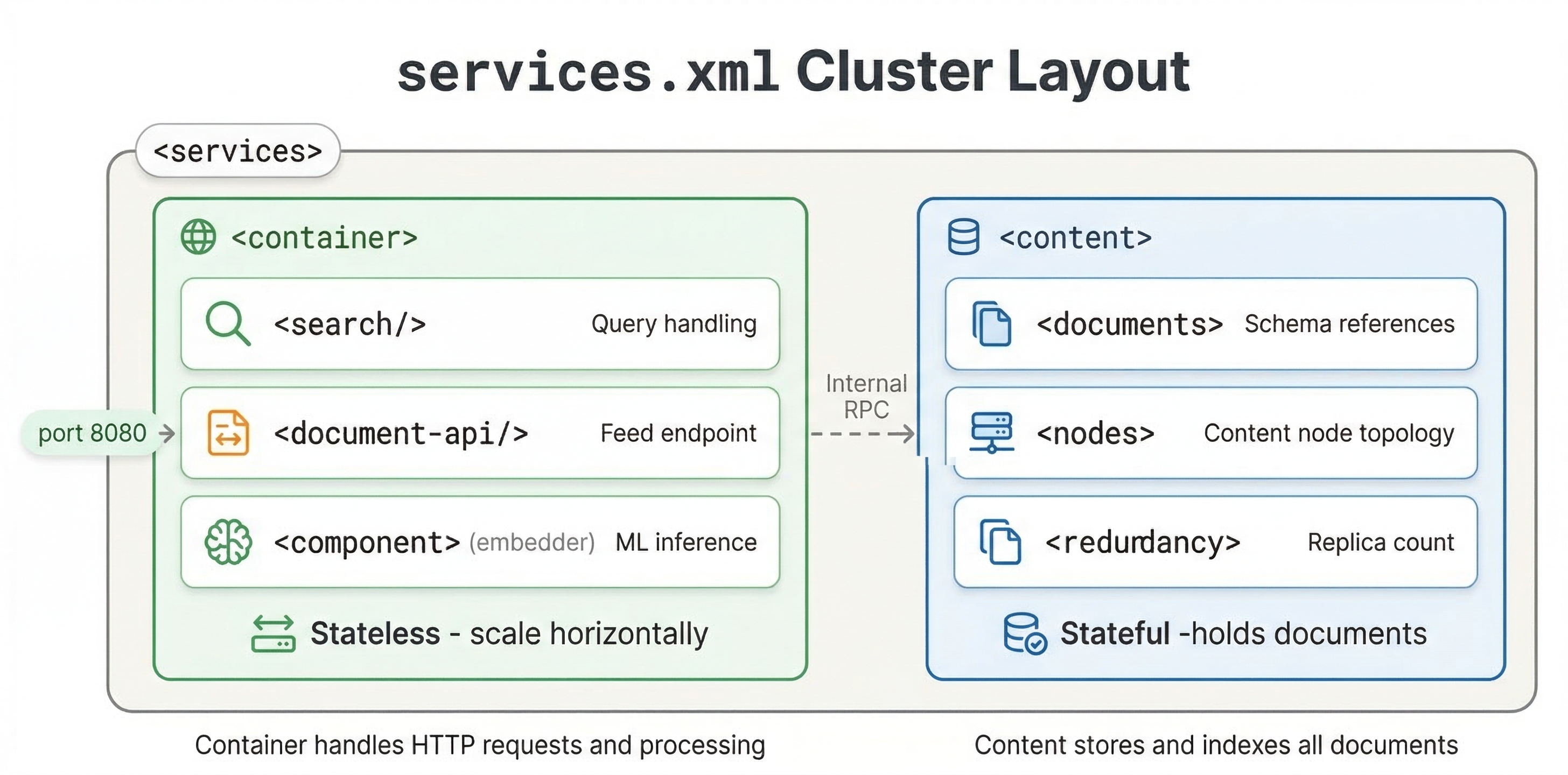
The services.xml file is where you define your cluster topology and configure how Vespa allocates resources and distributes work. Understanding how to configure clusters properly is essential for building applications that perform well and scale appropriately. In this chapter, we explore container and content cluster configuration, different topology patterns, and resource tuning.

Container Clusters

Container clusters are the stateless layer that handles queries, document processing, and custom application logic. You define container clusters in the <container> section of services.xml.

A basic container cluster looks like:

<container id="default" version="1.0">
  <search/>
  <document-api/>
  <nodes>
    <node hostalias="node1"/>
  </nodes>
</container>

The id attribute names the cluster. The <search/> component enables query processing. The <document-api/> component enables document feeding. The <nodes> section lists which hosts run this container.

You can run multiple container clusters if you want to separate concerns. For example, you might have one cluster for queries and another for document processing:

<container id="query" version="1.0">
  <search/>
  <nodes>
    <node hostalias="query1"/>
    <node hostalias="query2"/>
  </nodes>
</container>

<container id="feed" version="1.0">
  <document-api/>
  <nodes>
    <node hostalias="feed1"/>
  </nodes>
</container>

This separation lets you scale query and feeding capacity independently.

Content Clusters

Content clusters are the stateful layer that stores and indexes documents. You define them in the <content> section:

<content id="content" version="1.0">
  <redundancy>2</redundancy>
  <documents>
    <document type="product" mode="index"/>
  </documents>
  <nodes>
    <node distribution-key="0" hostalias="content1"/>
    <node distribution-key="1" hostalias="content2"/>
  </nodes>
</content>

The redundancy setting controls how many copies of each document are kept. With redundancy 2, each document is stored on 2 different nodes. This provides fault tolerance. If one node fails, the data is still available on another node.

The <documents> section lists which document types this content cluster stores. The mode="index" means documents are indexed and searchable. You can also use mode="streaming" for streaming search where documents are not pre-indexed, or mode="store-only" to store documents without indexing.

Each node needs a unique distribution-key. Vespa uses this to determine which documents go on which nodes. The keys must be unique integers and should be contiguous starting from 0 for a fresh system.

Single Node vs Multi-Node Topologies

For local development, a single-node topology is simplest:

<services version="1.0">
  <container id="default" version="1.0">
    <search/>
    <document-api/>
  </container>

  <content id="content" version="1.0">
    <redundancy>1</redundancy>
    <documents>
      <document type="product" mode="index"/>
    </documents>
    <nodes>
      <node distribution-key="0" hostalias="node1"/>
    </nodes>
  </content>
</services>

Notice we do not specify a <nodes> section in the container. When nodes are omitted, container services run on the same node as the config server. This works fine for development but is not production-ready.

For production, use multiple nodes for both containers and content:

<services version="1.0">
  <container id="default" version="1.0">
    <search/>
    <document-api/>
    <nodes>
      <node hostalias="container1"/>
      <node hostalias="container2"/>
    </nodes>
  </container>

  <content id="content" version="1.0">
    <redundancy>2</redundancy>
    <documents>
      <document type="product" mode="index"/>
    </documents>
    <nodes>
      <node distribution-key="0" hostalias="content1"/>
      <node distribution-key="1" hostalias="content2"/>
      <node distribution-key="2" hostalias="content3"/>
    </nodes>
  </content>
</services>

This configuration has 2 container nodes for query processing and 3 content nodes for data storage. With redundancy 2, each document exists on 2 of the 3 content nodes.

Resource Tuning

Vespa uses available memory and disk automatically, but you can tune resource allocation for specific needs.

For container clusters, you can set JVM heap size:

<container id="default" version="1.0">
  <search/>
  <nodes>
    <jvm allocated-memory="50%" />
    <node hostalias="container1"/>
  </nodes>
</container>

The <jvm> element configures the container JVM. The allocated-memory attribute controls what percentage of available memory is allocated to the JVM heap. The default is based on available system memory, but explicit settings help ensure consistent behavior.

For content clusters, you can configure how much memory to use for attribute data:

<content id="content" version="1.0">
  <engine>
    <proton>
      <tuning>
        <searchnode>
          <summary>
            <store>
              <cache>
                <maxsize>1073741824</maxsize>
              </cache>
            </store>
          </summary>
        </searchnode>
      </tuning>
    </proton>
  </engine>
  <redundancy>2</redundancy>
  <documents>
    <document type="product" mode="index"/>
  </documents>
  <nodes>
    <node distribution-key="0" hostalias="content1"/>
  </nodes>
</content>

These tuning options let you optimize memory usage for your data characteristics. Most applications work fine with defaults, but tuning helps when you have specific memory constraints or very large datasets.

Thread Pool Configuration

Container clusters use thread pools to handle concurrent queries. You can configure thread pool sizes:

<container id="default" version="1.0">
  <search>
    <threadpool>
      <threads>200</threads>
    </threadpool>
  </search>
  <nodes>
    <node hostalias="container1"/>
  </nodes>
</container>

The thread pool size determines how many queries can execute concurrently. Too few threads and you cannot utilize all CPU cores. Too many threads and you waste memory and CPU on context switching. The default based on CPU count works well for most applications.

Data Distribution and Groups

For large datasets, you can distribute data across multiple groups of nodes. This is called grouped distribution:

<content id="content" version="1.0">
  <redundancy>2</redundancy>
  <documents>
    <document type="product" mode="index"/>
  </documents>
  <group>
    <distribution partitions="1|*"/>
    <group distribution-key="0" name="group0">
      <node distribution-key="0" hostalias="content1"/>
      <node distribution-key="1" hostalias="content2"/>
    </group>
    <group distribution-key="1" name="group1">
      <node distribution-key="2" hostalias="content3"/>
      <node distribution-key="3" hostalias="content4"/>
    </group>
  </group>
</content>

This creates 2 groups with 2 nodes each. The partitions="1|*" setting means one copy goes to one group and the remaining copies go to another, distributing data across groups. Within each group, documents are replicated according to the redundancy setting. This topology scales to very large datasets while maintaining reasonable query latency.

Searchable Copies

You already know that redundancy controls how many copies of each document exist. But there is a related setting that is easy to overlook: searchable-copies. This controls how many of those copies are fully indexed and ready to serve queries.

With redundancy 2 and searchable-copies 1, two copies of every document exist for fault tolerance, but only one copy is indexed and searchable. The second copy is stored but not kept in the ready state. This saves memory because maintaining a searchable index is the expensive part.

With redundancy 2 and searchable-copies 2, both copies are fully indexed. Queries can hit either copy, which effectively doubles your query capacity. The trade-off is that both nodes now use memory for the full index.

Here is an example with explicit min-redundancy to control behavior during node failures:

<content id="content" version="1.0">
  <redundancy>2</redundancy>
  <min-redundancy>1</min-redundancy>
  <documents>
    <document type="product" mode="index"/>
  </documents>
  <nodes>
    <node distribution-key="0" hostalias="content1"/>
    <node distribution-key="1" hostalias="content2"/>
  </nodes>
</content>

The min-redundancy setting tells Vespa the minimum number of copies that must exist before it considers a write successful. Setting it to 1 means writes complete even if only one copy is confirmed, which keeps feeding fast during transient failures.

For most applications, searchable-copies equals redundancy, which is the default. You only need to lower searchable-copies when you want fault tolerance (extra copies of the data) but do not need the extra query capacity. This is common for write-heavy workloads where you want data safety without paying the memory cost of multiple searchable indexes.

Local vs Cloud Deployment

The services.xml structure is similar for local and cloud deployments, but there are differences in how you specify node counts.

For local deployment, you explicitly list nodes with hostaliases that map to actual hosts in hosts.xml. For Vespa Cloud, you specify node counts and resources, and the cloud platform allocates hosts:

<container id="default" version="1.0">
  <search/>
  <nodes count="2">
    <resources vcpu="4" memory="16Gb" disk="100Gb"/>
  </nodes>
</container>

The count attribute tells Vespa Cloud how many nodes you want. The <resources> element specifies CPU, memory, and disk for each node. Vespa Cloud provisions the requested resources automatically.

Monitoring and Status

After you deploy your application, you want to know that everything is running correctly. Vespa provides several tools for checking health and tracking performance.

The simplest check is vespa status, which tells you whether all services are up and healthy. Run it right after deployment to confirm everything started properly. If a service fails to start, you will see it here before any user traffic hits an error.

The config server exposes a status API on port 19071. You can hit http://<config-host>:19071/state/v1/health to check the config server itself. This is useful in automated health checks and deployment pipelines.

For runtime metrics, Vespa exposes a metrics endpoint at /metrics/v2/values on your container port (typically 8080). This gives you a JSON payload with metrics across all services, covering everything from query latency to memory usage. For production monitoring with Prometheus, use the /prometheus/v1/values endpoint instead. It serves the same data in a format Prometheus can scrape directly.

The metrics you should watch most closely are:

• Query latency (content.proton.documentdb.matching.rank_profile.query_latency), broken down by rank profile. This separation is valuable because it lets you track different query types independently, for example, user-facing searches vs automated background queries.
• Document count (content.proton.documentdb.documents.active), to confirm feeding is working and no documents are unexpectedly disappearing.
• Memory usage, especially attribute memory. If you are close to the limit, queries may slow down or fail.
• Disk usage, particularly for the document store and transaction log.

For Vespa Cloud deployments, metrics integrate with Grafana dashboards out of the box, giving you a visual overview without any setup on your side.

Two command-line tools are especially helpful for debugging cluster issues. vespa-model-inspect lets you find which ports services are running on and how the cluster is configured. If you are not sure where a service lives, this is the tool to reach for. vespa-sentinel-cmd checks the status of individual services on a node, which is useful when you need to diagnose whether a specific process has crashed or is misbehaving.

Best Practices

Start simple and add complexity as needed. A single content cluster and single container cluster work for most applications. Only create multiple clusters if you have a clear reason.

Size redundancy appropriately. Redundancy 2 provides good fault tolerance for production. Redundancy 1 is fine for development. Redundancy 3+ is typically only needed for very high availability requirements.

Plan for growth. If you start with 3 content nodes, adding more later requires data redistribution. Consider starting with more nodes than immediately needed if you expect growth.

Monitor resource usage. Watch memory, CPU, and disk usage on your nodes. If you are consistently near limits, add capacity before performance degrades.

Use Vespa Cloud for production if possible. The managed service handles cluster configuration, node provisioning, and capacity planning for you. This lets you focus on your application rather than infrastructure.

Next Steps

You now understand how to configure clusters for different topologies and resource requirements. The next chapter is a hands-on lab where you will modify an application package, add new configuration, and redeploy to see changes take effect.

For detailed configuration options, see the services.xml reference and Vespa sizing guides.