Multi-phase ranking and re-ranking

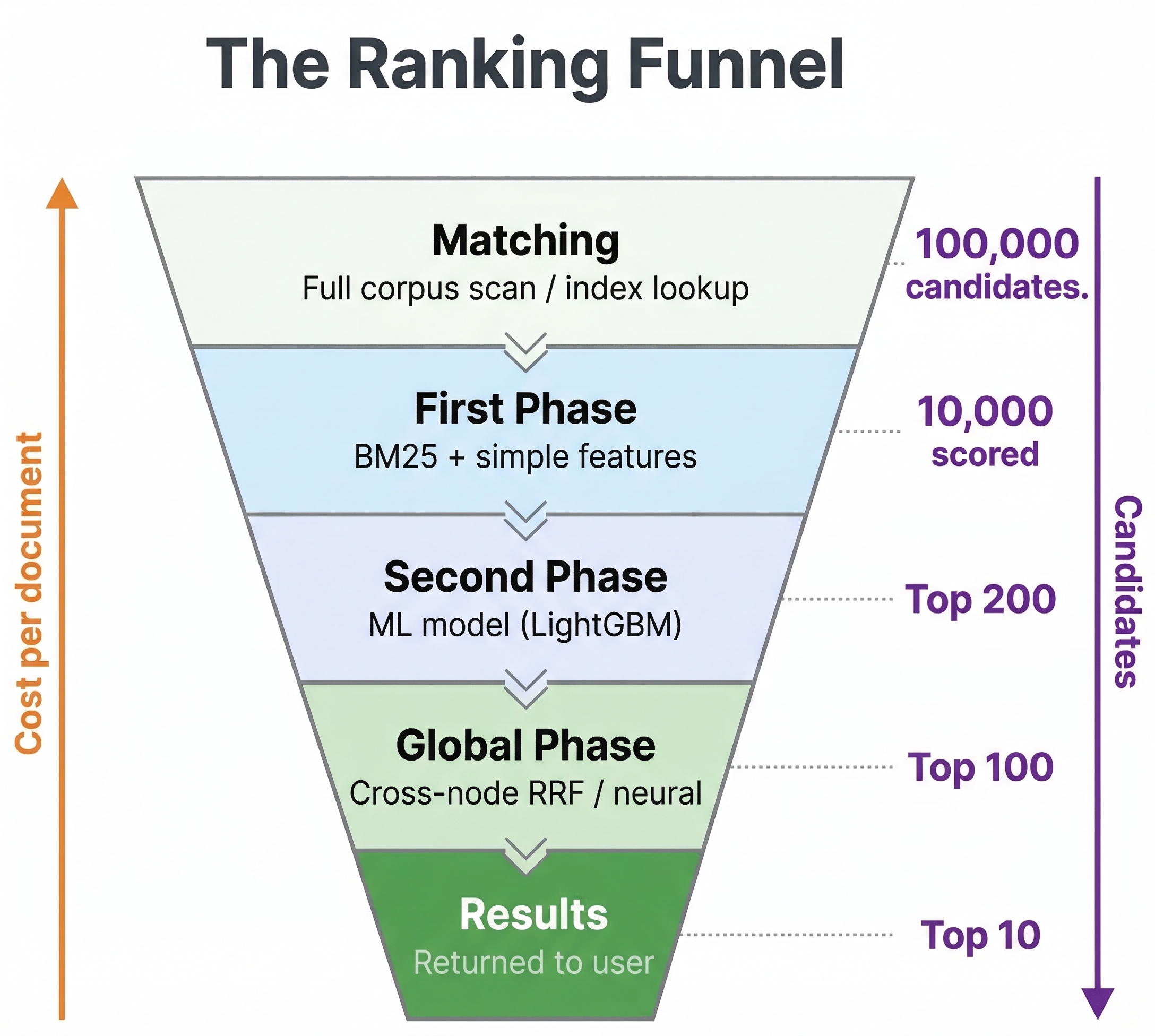
In previous modules, we defined rank profiles with a first-phase expression and briefly mentioned second-phase ranking. But ranking in Vespa is actually a multi-stage pipeline, and understanding this pipeline is essential for building search systems that are both fast and highly relevant. The core idea is simple: use a cheap function to score all matching documents, then apply progressively more expensive and accurate functions to smaller and smaller sets of top candidates. This way, you get the quality of expensive ranking without paying the cost of running it on every document.

In this chapter, we look at the full ranking pipeline in Vespa, from match-phase limiting all the way through global-phase re-ranking. We explore how each stage works, where it runs, and how to configure it. By the end, you will understand how to design ranking pipelines that balance latency and relevance for real production workloads.

The ranking pipeline

Vespa's ranking pipeline has several stages. Let's walk through the full journey of a query.

When a query arrives at a container node, it gets distributed to all content nodes that hold the data. Each content node finds the documents matching the query using retrieval operators like text matching, WAND, or nearest neighbor search. From here, the documents pass through up to four stages:

1. Match-phase limiting (optional) - a pre-first-phase optimization that caps how many documents even enter ranking
2. First-phase ranking - a fast expression that scores all matched documents on each content node
3. Second-phase ranking (optional) - a more expensive expression that re-ranks the top N documents per content node
4. Global-phase ranking (optional) - runs on the container node after results from all content nodes are merged

The first two stages always run on the content nodes where the data lives. This is important because content nodes have direct access to document attributes and tensors in memory, making computation fast. The global-phase runs on the container node, which sees the merged result set from all content nodes.

Let's look at each stage in detail.

First-phase ranking

First-phase ranking runs on every document that matches the query on each content node. Because it evaluates potentially millions of documents, the expression must be computationally cheap. This is not the place for neural network models or complex tensor operations.

Good first-phase expressions use fast features like BM25 text relevance, simple attribute lookups, and basic arithmetic:

rank-profile production {
    first-phase {
        expression: bm25(title) * 2 + bm25(body) + attribute(popularity) * 0.1
    }
}

This combines text relevance across two fields with a popularity signal. Each of these features is cheap to compute, so even millions of evaluations stay fast.

The first-phase has two additional configuration options that control how many documents survive to the next stage:

rank-profile production {
    first-phase {
        expression: bm25(title) + bm25(body)
        keep-rank-count: 10000
        rank-score-drop-limit: -1.0
    }
}

The keep-rank-count parameter controls how many top-scoring documents are retained per content node after first-phase ranking. The default is 10000. Documents that do not make it into this set are dropped entirely. If your second-phase only re-ranks 100 documents, keeping 10000 might seem excessive, but it provides a safety margin and allows for more accurate global merging.

The rank-score-drop-limit sets a score threshold. Documents scoring at or below this value are discarded regardless of keep-rank-count. This is useful for filtering out clearly irrelevant documents early. For example, if your first-phase uses BM25 and a document scores -1.0, it is almost certainly not relevant.

Second-phase ranking

Second-phase ranking is where you can bring in heavier computation. It runs on each content node, but only on the top N documents from the first phase. The number of documents is controlled by rerank-count, which defaults to 100 per content node.

rank-profile with_model {
    first-phase {
        expression: bm25(title) + bm25(body)
    }
    second-phase {
        expression: xgboost("my-model.json")
        rerank-count: 200
    }
}

In this example, the first phase scores all matches with BM25. Then the top 200 documents per content node get re-ranked using an XGBoost model. The XGBoost model can use many more features and capture complex interactions between them, producing much better relevance scores. But running it on 200 documents is very different from running it on 200,000.

Because second-phase runs on content nodes, it has efficient local access to all document data. This makes it the ideal place for machine learning models like XGBoost or LightGBM that need to read many document attributes. It is also suitable for moderately expensive ONNX models, though very large neural models might be better suited for the global-phase where you can use GPU acceleration.

You can also set a rank-score-drop-limit on the second phase:

second-phase {
    expression: xgboost("my-model.json")
    rerank-count: 200
    rank-score-drop-limit: 0.0
}

This drops any documents that score zero or below after second-phase evaluation, further trimming the result set before it gets sent to the container.

How rerank-count affects results

Understanding rerank-count is important for getting good results. If you have 10 content nodes and set rerank-count: 100, each content node re-ranks its local top 100 documents. The container then merges the results from all 10 nodes and returns the globally best ones.

Here is the subtle part: a document that ranked 101st on one content node never gets re-ranked, even if it would have scored highly in the second phase. If your first-phase ranking is not a good predictor of second-phase ranking, you might miss good documents. This is why having a reasonable first-phase expression matters. It does not need to be perfect, but it should roughly correlate with final relevance so the best candidates make it through.

If you find that increasing rerank-count significantly changes your top results, it means your first phase is not doing a great job of surfacing the right candidates. Consider improving it or increasing rerank-count at the cost of higher latency.

Global-phase ranking

Global-phase is the newest addition to Vespa's ranking pipeline. It runs on the container node after results from all content nodes have been merged. This gives it a unique capability: it sees the globally best results, not just the best from a single content node.

rank-profile with_global {
    first-phase {
        expression: bm25(title) + bm25(body)
    }
    second-phase {
        expression: xgboost("my-model.json")
        rerank-count: 200
    }
    global-phase {
        expression: normalize_linear(secondPhase) + query(boost) * attribute(priority)
        rerank-count: 100
    }
}

The global-phase rerank-count controls how many of the globally merged top results get re-ranked. The default is 100. You can also override this per-query using the ranking.globalPhase.rerankCount query parameter.

Cross-hit normalization functions

The most powerful feature of global-phase is cross-hit normalization. In earlier phases, each document is scored independently. But in the global phase, you can normalize scores across all the top hits. Vespa provides built-in functions for this:

normalize_linear(expression) scales scores to the range [0, 1] using min-max normalization. It computes (score - min) / (max - min) across all hits in the global-phase set. This is useful when combining scores from different sources that have different scales.

reciprocal_rank(expression) converts scores to rank-based values using the formula 1.0 / (k + rank) where k defaults to 60. You can customize k: reciprocal_rank(expression, 100). This is useful because it only cares about the ordering, not the absolute score values.

reciprocal_rank_fusion(a, b, c, ...) is a convenience function that sums individual reciprocal rank values across multiple scoring functions. This is the classic RRF approach popular in hybrid search.

Here is a typical hybrid search pattern using global-phase:

rank-profile hybrid {
    function bm25_score() {
        expression: bm25(title) + bm25(body)
    }

    function semantic_score() {
        expression: closeness(field, embedding)
    }

    first-phase {
        expression: bm25_score + semantic_score
    }

    global-phase {
        rerank-count: 200
        expression: reciprocal_rank_fusion(bm25_score, semantic_score)
    }
}

The first-phase does a rough combination of text and semantic scores. Then the global-phase applies reciprocal rank fusion, which normalizes both signals into rank-based scores and combines them. This often produces better results than trying to manually weight raw BM25 scores against cosine similarity scores, because those two live on completely different scales.

When to use global-phase

Global-phase is the right choice when you need to:

• Normalize scores across different signals. BM25 scores and vector similarity scores have different ranges. Global-phase normalization puts them on the same scale.
• Apply cross-encoder models. Large transformer models that score query-document pairs are very expensive. Running them on 25-100 globally best documents in the global-phase (potentially with GPU acceleration) is practical.
• Enforce result diversity. Since global-phase sees the full merged result set, it can ensure diverse categories, sources, or other attributes across results.
• Apply business rules that need the full picture. Promoting certain results or enforcing positional constraints works best when you see all candidates together.

GPU support in global-phase

For expensive ONNX model inference in global-phase, Vespa supports GPU acceleration:

rank-profile cross_encoder_gpu {
    onnx-model cross_encoder {
        file: models/cross-encoder.onnx
        input input_ids: my_input_ids
        input attention_mask: my_attention_mask
        gpu-device: 0
    }

    first-phase {
        expression: bm25(title)
    }

    global-phase {
        rerank-count: 25
        expression: onnx(cross_encoder){d0:0,d1:0}
    }
}

This runs the cross-encoder on a GPU attached to the container node, but only for the top 25 globally merged results. Even a large cross-encoder model can score 25 documents quickly on a GPU.

Match-phase limiting

Match-phase limiting is a performance optimization that sits before first-phase ranking. When a query matches a very large number of documents, even a cheap first-phase expression can become slow if it has to score millions of hits. Match-phase limiting caps the number of documents that enter ranking by filtering based on a document quality attribute.

rank-profile with_limiting {
    match-phase {
        attribute: popularity
        order: descending
        max-hits: 10000
    }
    first-phase {
        expression: bm25(title) + attribute(popularity) * 0.1
    }
}

The attribute must be a single-valued numeric field with fast-search enabled. The order specifies whether higher or lower values are preferred. The max-hits is the target number of candidates. When the system estimates that a query matches more documents than max-hits, it implicitly filters to keep only documents with the best attribute values.

For the attribute to work with match-phase, your schema needs:

field popularity type int {
    indexing: summary | attribute
    attribute: fast-search
}

Match-phase limiting is a powerful optimization, but it comes with important caveats. It works well for broad queries that match many documents. But when combined with restrictive filters, it can actually increase latency. If few documents pass both the query filter and the match-phase quality threshold, the system has to evaluate many documents before finding enough candidates. This creates the counterintuitive situation where more restrictive queries become slower.

Use match-phase limiting when your typical queries match tens of thousands or more documents, and when you have a meaningful quality attribute that correlates with what users want. Monitor the content.proton.documentdb.matching.rank_profile.limited_queries metric to see how often limiting kicks in.

Match-features and summary-features

When building a multi-phase ranking pipeline, you often need to inspect the features used at each stage. Vespa provides two mechanisms for this: match-features and summary-features.

Match-features

Match-features are computed during first-phase ranking for all matched hits. They are returned with each hit and are available in subsequent ranking phases. This has an important practical use: if your global-phase needs values that are expensive to compute and require local data access, you can declare them as match-features. They get computed on the content node (where the data lives) and transferred to the container as pre-computed values.

rank-profile efficient_global {
    function text_score() {
        expression: bm25(title) * 2 + bm25(body)
    }

    function vector_score() {
        expression: closeness(field, embedding)
    }

    match-features: text_score vector_score

    first-phase {
        expression: text_score + vector_score
    }

    global-phase {
        rerank-count: 200
        expression: normalize_linear(text_score) + normalize_linear(vector_score)
    }
}

In this example, text_score and vector_score are computed on the content nodes during first-phase. When these hits reach the container for global-phase, the pre-computed values are used instead of trying to recompute them (which would be impossible since the container does not have local access to document data). This pattern is essential for efficient global-phase ranking.

Match-features also appear in the search results, making them useful for debugging and logging.

Summary-features

Summary-features are computed only for the final set of returned hits, during the summary fill phase. They are more efficient than match-features when you only need values for display or logging, not for ranking decisions.

rank-profile with_logging {
    summary-features: bm25(title) bm25(body) attribute(popularity) firstPhase secondPhase

    first-phase {
        expression: bm25(title) + bm25(body)
    }
    second-phase {
        expression: xgboost("my-model.json")
        rerank-count: 100
    }
}

The firstPhase and secondPhase summary features return the scores from each ranking phase, which is invaluable for debugging why a document ranked where it did. You can also log these features for building training data for learning-to-rank models, which we cover in the next chapter.

Designing a ranking pipeline

Now that you understand each stage, let's talk about how to put them together. The general principle is a funnel: start wide with cheap computation and narrow down with expensive computation.

A practical example

Imagine you are building a product search for an e-commerce site. You have text fields (title, description), a popularity score, category attributes, and vector embeddings. Here is how you might design the pipeline:

rank-profile ecommerce_search {
    match-phase {
        attribute: popularity
        order: descending
        max-hits: 50000
    }

    function text_relevance() {
        expression: bm25(title) * 3 + bm25(description)
    }

    function semantic_relevance() {
        expression: closeness(field, embedding)
    }

    match-features: text_relevance semantic_relevance attribute(popularity) attribute(in_stock)

    first-phase {
        expression: text_relevance + semantic_relevance * 10 + if(attribute(in_stock), 5, 0)
    }

    second-phase {
        expression: xgboost("product-ranker.json")
        rerank-count: 200
    }

    global-phase {
        rerank-count: 100
        expression {
            reciprocal_rank_fusion(text_relevance, semantic_relevance) +
            if(attribute(in_stock), 0.1, 0)
        }
    }
}

Here is what happens at each stage:

1. Match-phase limits candidates to the top 50,000 by popularity if the query is very broad.
2. First-phase scores all remaining matches with a combination of text, semantic, and in-stock signals. This is fast but rough.
3. Second-phase re-ranks the top 200 per content node using an XGBoost model that captures complex feature interactions.
4. Global-phase applies reciprocal rank fusion on the merged results, normalizing text and semantic scores properly, and gives a final boost to in-stock items.

Each stage applies progressively better ranking while keeping total latency acceptable.

Choosing what goes where

Here are some guidelines for deciding which ranking logic belongs in which phase:

First-phase: BM25, nativeRank, simple attribute arithmetic, basic freshness calculations. Anything that computes in microseconds per document.

Second-phase: Machine learning models (XGBoost, LightGBM), moderately complex tensor operations, ONNX models that can handle hundreds of evaluations per query. Runs on content nodes with local data access.

Global-phase: Cross-hit normalization (RRF, linear normalization), expensive cross-encoder models on small candidate sets, diversity enforcement, business rules that need the full result picture. Runs on the container node.

Re-ranking strategies beyond relevance

Multi-phase ranking is not only about improving relevance. The later phases, especially global-phase, are perfect for applying non-relevance signals.

Business rules

Promote or demote results based on business logic. Sponsored products should appear in specific positions. Certain categories should be boosted during seasonal events.

global-phase {
    rerank-count: 50
    expression {
        secondPhase +
        if(attribute(is_sponsored), 100, 0) +
        if(attribute(is_seasonal_promo), 50, 0)
    }
}

Personalization

If you pass user preference signals as query features, later phases can incorporate them:

second-phase {
    expression {
        bm25(title) +
        sum(query(user_category_preferences) * attribute(category_vector))
    }
    rerank-count: 200
}

This computes a dot product between user preferences and document category vectors, personalizing the results for each user.

Diversification

Vespa supports result diversity as a built-in feature that works alongside the ranking pipeline:

rank-profile diverse_results {
    diversity {
        attribute: category
        min-groups: 5
    }
    first-phase {
        expression: bm25(title)
    }
}

This ensures that results come from at least 5 different categories, preventing a single dominant category from taking all top positions.

Performance tuning

Multi-phase ranking gives you direct control over the latency-quality tradeoff. Here are the main levers:

Reduce rerank-count in second-phase. Going from 200 to 50 cuts second-phase computation by 75%. Test whether this noticeably hurts result quality for your use case.

Reduce rerank-count in global-phase. Same idea. Fewer documents in global-phase means less data transferred from content nodes and less computation on the container.

Tune keep-rank-count in first-phase. The default of 10,000 is conservative. If your second-phase rerank-count is 100, keeping 1,000 might be sufficient and reduces memory usage.

Use match-phase limiting for broad queries. If your typical queries match hundreds of thousands of documents, match-phase limiting can dramatically reduce first-phase evaluation count.

Pre-compute for global-phase using match-features. Declare expensive functions as match-features so they run on content nodes. The global-phase then works with pre-computed scalar values instead of trying to access raw document data.

Tune threading. Vespa can parallelize first-phase ranking across multiple threads per search:

rank-profile fast {
    num-threads-per-search: 4
    min-hits-per-thread: 100
    first-phase {
        expression: bm25(title)
    }
}

More threads help when you have many documents to score and available CPU cores.

A note on Vespa Cloud vs local

Everything in this chapter works the same way whether you run Vespa locally or on Vespa Cloud. The ranking pipeline, configuration syntax, and behavior are identical. The main difference is operational: on Vespa Cloud, you do not manage the content and container nodes yourself. The platform handles scaling, and you can configure GPU resources for global-phase through the Vespa Cloud console. Locally, you would need to set up GPU passthrough in your container or bare-metal environment if you want GPU-accelerated global-phase inference.

Next steps

You now understand Vespa's full multi-phase ranking pipeline. You know how to use first-phase for fast candidate scoring, second-phase for ML model re-ranking on content nodes, and global-phase for cross-hit normalization and final re-ranking on the container. You also know how to use match-phase limiting for performance and match-features to bridge data between content and container nodes.

In the next chapter, we dive into learning to rank with gradient-boosted decision tree models. You will learn how to train XGBoost and LightGBM models and deploy them in Vespa's second-phase ranking.

For complete details on phased ranking, see the Vespa phased ranking documentation. For cross-encoder re-ranking patterns, see the cross-encoder guide.