Generating and using training data

Learning to rank is only as good as the data you train on. You can have the most sophisticated model architecture, but if your training data is noisy, biased, or incomplete, the model will learn the wrong things. In this chapter, we cover how to collect ranking features from Vespa, how to derive relevance labels from user behavior, and how to build high-quality training datasets for your LTR models.

This is arguably the most important chapter in the module. Getting training data right is where most of the effort goes in a real LTR system, and it is where the biggest improvements come from.

Logging ranking features from Vespa

The first step in building training data is extracting the features that your model will use. Vespa provides several mechanisms for this.

Summary-features

Summary-features are computed during the fill phase, meaning only for the final set of results returned to the user. This is efficient because you only compute features for hits that matter:

rank-profile production_with_logging {
    first-phase {
        expression: bm25(title) + bm25(body)
    }
    second-phase {
        expression: xgboost("current_model.json")
        rerank-count: 200
    }
    summary-features {
        bm25(title)
        bm25(body)
        nativeRank(title)
        nativeRank(body)
        fieldMatch(title)
        fieldMatch(title).proximity
        fieldMatch(title).completeness
        attribute(popularity)
        freshness(timestamp)
        closeness(field, embedding)
        firstPhase
        secondPhase
    }
}

The firstPhase and secondPhase special features return the scores from each ranking phase. These are useful for debugging and for understanding how the current model is scoring documents.

Summary-features appear in the search results under a summaryfeatures field in each hit. Your application can log these alongside the query, document ID, and position for later training.

Match-features

Match-features are computed during first-phase ranking for all matched hits. They are more expensive than summary-features because they apply to every hit, not just the final results. But they have an important advantage: they are available to subsequent ranking phases and can be used in global-phase re-ranking.

rank-profile with_match_features {
    match-features {
        bm25(title)
        bm25(body)
        attribute(popularity)
        closeness(field, embedding)
    }
    first-phase {
        expression: bm25(title) + bm25(body)
    }
}

For training data collection, match-features are useful when you want features for documents beyond just the top results. If a user clicks on a result at position 15, you need the features for that document too, and match-features ensure they are available.

The ranking.listFeatures parameter

For exploration and initial feature discovery, you can add ranking.listFeatures=true to any query. This returns all default rank features for each hit without needing to configure anything in the rank profile:

/search/?yql=select * from doc where title contains "laptop"
  &ranking.listFeatures=true
  &ranking.profile=my-profile

This dumps a large set of features per hit. It is useful for understanding what features Vespa computes and for deciding which ones to include in your model. Do not use this in production feature logging because it computes far more features than you need and adds significant overhead.

A dedicated feature collection rank profile

For systematic training data collection, create a dedicated rank profile that randomizes the first-phase ranking:

rank-profile collect_training_data {
    first-phase {
        expression: random
    }
    match-features {
        bm25(title)
        bm25(body)
        nativeRank(title)
        nativeRank(body)
        fieldMatch(title)
        fieldMatch(title).proximity
        fieldMatch(title).completeness
        fieldMatch(body)
        attribute(popularity)
        freshness(timestamp)
        closeness(field, embedding)
    }
}

Using random as the first-phase expression returns a random sample of matching documents rather than the top-ranked ones. This is important because training data needs both relevant and irrelevant examples. If you only collect features for top-ranked documents, your training data will be biased toward documents that the current system already ranks highly.

Deriving relevance labels

Features are half the equation. The other half is relevance labels: telling the model which documents are good for which queries. There are two main sources of labels: human judgments and user behavior.

Human relevance judgments

Human assessors look at query-document pairs and assign a relevance grade. This is the gold standard for label quality. A typical grading scale is:

• 0 - Irrelevant: The document has nothing to do with the query
• 1 - Marginally relevant: The document touches on the topic but does not answer the query
• 2 - Relevant: The document is about the right topic and partially answers the query
• 3 - Highly relevant: The document directly and thoroughly answers the query

Some systems use a 5-point scale (0-4). The exact number of grades matters less than having clear definitions with examples for each grade level.

Human judgments are expensive to produce. A single assessor might judge 200-400 query-document pairs per day. To get reliable labels, you typically want 2-3 assessors per pair and use majority vote or averaging to handle disagreements. Measure inter-annotator agreement (using metrics like Cohen's kappa) to ensure your guidelines are clear enough.

Despite the cost, human judgments are essential for creating evaluation test sets. Even if you train on click data, you should evaluate on human-labeled data to measure true relevance improvements.

Click-based labels

User clicks are a cheaper and more abundant source of relevance signals. Every search session generates implicit feedback: which results the user clicked, how long they spent on each result, whether they returned to the search results page, and what they did next.

The simplest approach is binary: a clicked document is labeled relevant (1) and everything else is labeled irrelevant (0). This works as a starting point but is quite noisy. Users click for many reasons beyond relevance, including curiosity, attractive titles, or just position on the page.

A better approach uses multiple behavioral signals to assign graded labels:

• No interaction: label 0
• Click with short dwell time (under 10 seconds, the user bounced back quickly): label 1
• Click with moderate dwell time (10-30 seconds): label 2
• Click with long dwell time (over 30 seconds, the user engaged with the content): label 3

For e-commerce, you can use conversion signals:

• No interaction: label 0
• Click: label 1
• Add to cart: label 2
• Purchase: label 3

The specific thresholds and mappings depend on your domain. The key principle is that stronger engagement signals should correspond to higher relevance grades.

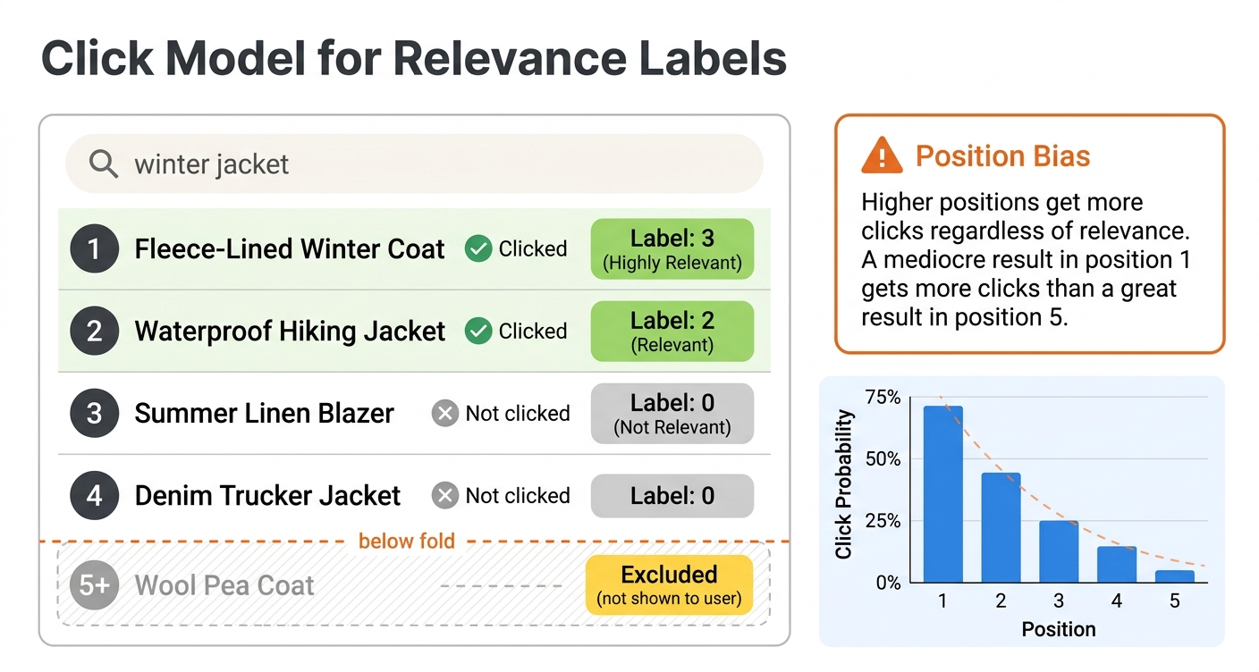
Handling position bias

The biggest challenge with click-based labels is position bias. Users are much more likely to click results at higher positions simply because they see them first. A mediocre result at position 1 gets more clicks than a great result at position 8, not because it is more relevant but because it is more visible.

If you ignore position bias, your model learns to replicate the current ranking rather than improve it. Results that are already ranked highly get more clicks, which generates more positive labels, which reinforces their high ranking. This creates a feedback loop that prevents improvement.

The standard solution is inverse propensity scoring (IPS). The idea is to weight each click by the inverse of its examination probability. If position 1 has a 90% chance of being examined and position 10 has a 20% chance, a click at position 10 is weighted 4.5 times more than a click at position 1. This corrects for the fact that lower-position clicks are more informative.

To estimate position propensities, you can run a small randomization experiment. For a fraction of traffic, randomly shuffle the top results. Since position is randomized, differences in click rates between positions reflect true examination probabilities rather than relevance differences. Once you have propensity estimates, apply IPS weighting when building your training labels.

A simpler alternative is to only use relative comparisons within the same query. If the user clicked result at position 5 but skipped results at positions 1-4, this tells you something about relative relevance regardless of absolute position bias. This "skip-above" signal is less affected by position bias because all the documents in the comparison were visible to the user.

Building the training dataset

Once you have features and labels, you need to assemble them into the format expected by your ranking model.

Data format

Both XGBoost and LightGBM expect training data organized by query groups. Each row is a query-document pair with a relevance label and feature values. Documents belonging to the same query must be grouped together.

In Python, the typical structure is a DataFrame:

import pandas as pd

# Each row: query_id, doc_id, label, feature_1, feature_2, ...
df = pd.DataFrame({
    'query_id': [1, 1, 1, 2, 2, 2, 2],
    'doc_id': ['a', 'b', 'c', 'd', 'e', 'f', 'g'],
    'label': [3, 0, 1, 2, 3, 0, 1],
    'bm25_title': [4.2, 0.0, 1.1, 3.8, 5.1, 0.3, 2.0],
    'bm25_body': [2.1, 0.5, 0.8, 1.9, 3.2, 0.1, 1.5],
    'popularity': [850, 120, 300, 500, 920, 50, 400],
    'freshness': [0.9, 0.3, 0.7, 0.8, 0.95, 0.1, 0.6],
})

# Group sizes for the ranking objective
group_sizes = df.groupby('query_id').size().values  # [3, 4]

The group sizes array tells the model how many documents belong to each query. This is how LambdaMART knows which documents to compare when computing pairwise gradients.

Collecting features with PyVespa

PyVespa provides tools for collecting training data from a running Vespa instance. The basic workflow is:

from vespa.application import Vespa

app = Vespa(url="http://localhost", port=8080)

queries = {
    "q1": "best laptop for programming",
    "q2": "wireless noise canceling headphones",
    "q3": "ergonomic office chair",
}

relevant_docs = {
    "q1": ["doc-101", "doc-203", "doc-55"],
    "q2": ["doc-88", "doc-412"],
    "q3": ["doc-77", "doc-199", "doc-301"],
}

all_features = []

for qid, query_text in queries.items():
    response = app.query(
        yql="select * from product where userInput(@query)",
        query=query_text,
        ranking="collect_training_data",
        hits=50
    )

    for hit in response.hits:
        features = hit.get("matchfeatures", {})
        doc_id = hit["id"]
        label = 1 if doc_id in relevant_docs.get(qid, []) else 0

        row = {"query_id": qid, "doc_id": doc_id, "label": label}
        row.update(features)
        all_features.append(row)

df = pd.DataFrame(all_features)

This queries Vespa with the feature collection rank profile, extracts match-features from each hit, and builds a DataFrame with labels. For real training data, you would use more sophisticated labeling (human judgments or click-derived grades) rather than simple binary labels.

Including negative examples

A common mistake is only collecting features for documents that the user interacted with. Your model needs to see negative examples too, otherwise it has no contrast for learning what makes a document irrelevant.

The randomized rank profile approach helps: by using random as the first-phase expression, you get a diverse sample of matching documents, many of which are irrelevant. You can also explicitly sample random documents for each query:

# For each query, collect features for random matching documents
response = app.query(
    yql="select * from product where userInput(@query)",
    query=query_text,
    ranking="collect_training_data",
    hits=100  # Get more documents, most will be irrelevant
)

A good ratio is roughly 1 relevant document to 5-10 irrelevant documents per query. Too few negatives means the model does not learn to differentiate well. Too many can slow down training without adding much signal.

The recall parameter

For collecting features of specific documents that might not normally appear in search results, Vespa supports a recall parameter. This forces specific documents into the result set so you can get their features for any query:

/search/?yql=select * from product where userInput(@query)
  &query=laptop
  &ranking=collect_training_data
  &recall=+(id:doc-101 id:doc-203 id:doc-55)

This ensures that documents doc-101, doc-203, and doc-55 are included in the results regardless of how they match the query. The match features are still computed normally, so BM25 and other interaction features reflect the actual query-document relationship. This is particularly useful for getting features for human-judged documents that might rank too low to appear in normal results.

Feature engineering

Choosing the right features is as important as choosing the right model. Here are the most useful feature categories for LTR in Vespa.

Text matching features

These capture how well the query matches document text:

• bm25(field) - the standard BM25 relevance score. Fast and effective. Use it for every text field.
• nativeRank(field) - Vespa's normalized text match score combining multiple signals. A good default feature.
• fieldMatch(field) - a sophisticated text matching score that considers term proximity, ordering, and completeness. More expensive to compute than BM25 but often more informative.
• fieldMatch(field).proximity - how close the matched query terms appear in the document. Important for phrase-like queries.
• fieldMatch(field).completeness - what fraction of the query is matched in the field. Useful for detecting partial matches.
• fieldMatch(field).queryCompleteness - what fraction of query terms are found in the field.

Document quality features

These are independent of the query:

• attribute(popularity) - any numeric quality signal stored as a document attribute
• freshness(timestamp) - recency signal, decays over time
• attribute(rating) - user ratings, review scores
• attribute(price) - for e-commerce
• fieldLength(field) - document length, which can be a quality indicator

Semantic features

If you have vector embeddings:

• closeness(field, embedding) - semantic similarity from nearest neighbor search

Query features

Passed at query time:

• query(user_intent) - classified query intent
• query(category_preference) - user personalization signals
• queryTermCount - number of terms in the query

Feature selection tips

Start with 10-15 strong features and expand from there. A good starting set for a typical search application:

match-features {
    bm25(title)
    bm25(body)
    nativeRank(title)
    fieldMatch(title).completeness
    fieldMatch(title).proximity
    attribute(popularity)
    freshness(timestamp)
    closeness(field, embedding)
}

After training an initial model, use feature importance scores from XGBoost or LightGBM to identify which features contribute most. Drop features that have near-zero importance because they add complexity without improving the model.

Always extract features from Vespa itself rather than recomputing them offline. This is critical. If you compute BM25 in Python using a different implementation, the scores will not match what Vespa produces at serving time. This feature drift between training and inference will hurt your model's effectiveness. When your training DataFrame column names map directly to Vespa feature names, you have exact parity between training and serving.

Creating evaluation sets

You need a separate evaluation set to measure whether model changes actually improve ranking. This set should not overlap with your training data.

Golden queries

A golden query set is a curated collection of representative queries with thorough relevance judgments. These queries serve as your stable evaluation benchmark. A good golden set includes:

• Head queries (high frequency) - your most common queries, representing the bulk of traffic
• Torso queries (medium frequency) - important queries that are less common
• Tail queries (low frequency) - rare queries that test generalization
• Different intent types - navigational ("amazon"), informational ("how to tie a tie"), transactional ("buy running shoes")

For each golden query, you want comprehensive relevance judgments covering both highly relevant and irrelevant documents. This usually requires human annotation because click data is too sparse for rare queries.

Train/test split

When training, always hold out a portion of your data for evaluation:

from sklearn.model_selection import GroupShuffleSplit

splitter = GroupShuffleSplit(n_splits=1, test_size=0.2, random_state=42)
train_idx, test_idx = next(splitter.split(X, y, groups=query_ids))

X_train, X_test = X[train_idx], X[test_idx]
y_train, y_test = y[train_idx], y[test_idx]

Using GroupShuffleSplit with query IDs ensures that all documents for a query end up in either train or test, never split across both. This prevents data leakage where the model memorizes specific query-document relationships.

Monitoring evaluation metrics over time

Track your evaluation metrics across model iterations:

from sklearn.metrics import ndcg_score

# Compute NDCG@10 per query, then average
ndcg_scores = []
for qid in test_query_ids:
    mask = test_df['query_id'] == qid
    true_labels = test_df.loc[mask, 'label'].values
    predictions = model.predict(test_df.loc[mask, feature_cols].values)

    if len(true_labels) > 1 and sum(true_labels) > 0:
        score = ndcg_score([true_labels], [predictions], k=10)
        ndcg_scores.append(score)

mean_ndcg = sum(ndcg_scores) / len(ndcg_scores)
print(f"Mean NDCG@10: {mean_ndcg:.4f}")

Data quality considerations

Filtering bot traffic

Automated traffic (crawlers, scrapers, monitoring bots) generates click patterns that look nothing like real user behavior. Including bot traffic in your training data introduces noise. Filter by user agent, flag IP addresses with superhuman click rates, and remove sessions with zero dwell time on all clicks.

Handling sparse labels

For most queries, you will have very few labeled documents. A query might match thousands of documents but only have labels for 5-10 of them. This is normal. Unlabeled documents are typically treated as irrelevant (label 0), which introduces some noise but works well enough in practice.

For critical queries, supplement sparse click data with human judgments through active learning. Choose the query-document pairs where the model is most uncertain and send those for human annotation. This targets annotation effort where it has the most impact.

Temporal considerations

User behavior changes over time. Queries shift with seasons, trends, and current events. A model trained on last year's data may not perform well on today's queries. Retrain regularly with fresh data and monitor for performance degradation.

When aggregating click data, use consistent time windows. Aggregate over at least 2-4 weeks to get stable click-through rates. Short windows produce noisy estimates, especially for low-traffic queries.

Cold start for new documents

New documents have no behavioral features (no clicks, no popularity). Your model needs to handle this gracefully. One approach is to use content-based features (text quality, metadata) for new documents and transition to behavioral features as data accumulates. Another is to use a separate "cold start" rank profile with different feature weights until the document has enough history.

The training data flywheel

Once you have a working LTR system, it creates a positive feedback loop:

1. Better ranking leads to more user engagement
2. More engagement generates more click data
3. More click data improves training data quality
4. Better training data produces better models
5. Better models improve ranking

This flywheel means that the most important thing is to get started. Your first model does not need perfect training data. It just needs to be better than the hand-tuned baseline. As it improves ranking and generates more behavioral data, each subsequent model gets better.

Next steps

You now understand how to collect features from Vespa, derive relevance labels from user behavior, and build training datasets for LTR models. In the next chapter, we put it all together in a hands-on lab where you train a model and deploy it as a re-ranker.

For more on feature collection, see the Vespa rank features reference. For end-to-end examples, see the Vespa blog series on improving product search with LTR.