Learning to rank with GBDT models

In the previous chapter, we explored Vespa's multi-phase ranking pipeline. You saw how to use hand-tuned expressions combining BM25, freshness, and attribute signals. But manually choosing features and tuning weights only gets you so far. At some point, you want a machine learning model to learn the optimal combination of features from data. This is what learning to rank (LTR) is about.

Gradient-boosted decision tree (GBDT) models, specifically XGBoost and LightGBM, are the workhorses of learning to rank. They are fast to evaluate, easy to train, and remarkably effective at combining diverse features into a single relevance score. Vespa has native support for both frameworks, making it straightforward to train a model in Python and deploy it directly into your ranking pipeline.

In this chapter, we cover how LTR works conceptually, how to train XGBoost and LightGBM ranking models, and how to deploy them in Vespa rank profiles.

What is learning to rank

Learning to rank is the application of machine learning to the ranking problem. Instead of manually writing a scoring formula like bm25(title) * 2 + attribute(popularity) * 0.1, you train a model on labeled data. The model learns which features matter, how they interact, and what weights to assign, all from examples of good and bad rankings.

The basic idea is this: for a set of queries, you have documents with relevance labels (either from human judgments or from user behavior like clicks). You extract features for each query-document pair, things like BM25 scores, document popularity, field match quality, freshness, and so on. Then you train a model to predict relevance from these features. The trained model replaces your hand-tuned ranking expression.

LTR approaches

There are three main approaches to learning to rank, and they differ in how the training loss is defined:

Pointwise treats each document independently. The model learns to predict an absolute relevance score for a single document. This is essentially a regression or classification problem. It works, but it ignores the relative ordering between documents, which is what ranking is actually about.

Pairwise considers pairs of documents for the same query. The model learns that document A should rank above document B. The training signal comes from comparing document pairs. This directly optimizes ordering, which aligns better with the ranking task.

Listwise considers the entire list of documents for a query. The model directly optimizes list-level metrics like NDCG or MAP. This is the most sophisticated approach and generally produces the best results.

In practice, the distinction blurs. The most popular algorithm, LambdaMART (used by both XGBoost and LightGBM for ranking), is technically a hybrid. It computes pairwise gradients but scales them by the change in NDCG that would result from swapping two documents. The result is a model that effectively optimizes a list-level metric through pairwise comparisons. And the output is still a pointwise scoring function that scores one document at a time, which is exactly what Vespa needs for distributed evaluation.

Features for learning to rank

The features you use in your LTR model are what make or break its effectiveness. Features fall into three categories:

Query features

These depend only on the query, not on any particular document. Examples include query length, query type (navigational vs informational), time of day, or user context like location or preferences. In Vespa, you pass these as query-time features using query(name) parameters.

Document features

These depend only on the document, not on the query. Examples include document popularity, quality score, content length, recency, price, or category. In Vespa, you access these through attribute(field) in your ranking expressions.

Query-document features

These depend on the interaction between a specific query and a specific document. These are usually the most powerful features for ranking. Examples include BM25 scores, field match completeness, proximity of query terms in the document, and vector similarity scores. Vespa computes these automatically through rank features like bm25(field), fieldMatch(field).completeness, fieldMatch(field).proximity, and closeness(field, embedding).

A typical LTR model might use 20 to 50 features spanning all three categories. More features are not always better. Noisy or redundant features can hurt model quality and slow down evaluation. Start with the most informative features and add more incrementally.

Training an XGBoost ranking model

Let's walk through training an XGBoost model for ranking. We assume you have already collected training data with features and relevance labels. We cover how to collect that data in a later chapter. For now, focus on the training and deployment process.

Preparing the data

XGBoost expects a feature matrix, relevance labels, and group sizes. The group sizes tell XGBoost which documents belong to the same query, so it can compute pairwise and listwise losses correctly.

import xgboost as xgb
import numpy as np

# X_train: feature matrix, shape (num_docs, num_features)
# y_train: relevance labels (0-4 graded scale), shape (num_docs,)
# group_sizes: number of documents per query, e.g. [15, 23, 8, ...]

dtrain = xgb.DMatrix(X_train, label=y_train)
dtrain.set_group(group_sizes)

The relevance labels are typically on a graded scale: 0 means not relevant, 1 is marginally relevant, 2 is relevant, 3 is highly relevant, 4 is perfect. But binary labels (0 or 1) work too.

Training the model

For ranking, use the rank:ndcg objective, which implements LambdaMART optimizing NDCG:

params = {
    'objective': 'rank:ndcg',
    'max_depth': 5,
    'eta': 0.1,
    'eval_metric': 'ndcg@10',
    'base_score': 0
}

# If you have a validation set
dval = xgb.DMatrix(X_val, label=y_val)
dval.set_group(val_group_sizes)

model = xgb.train(
    params,
    dtrain,
    num_boost_round=200,
    evals=[(dtrain, 'train'), (dval, 'val')],
    early_stopping_rounds=20
)

Other useful objectives include rank:pairwise for pairwise logistic loss and rank:map for optimizing MAP (binary relevance only). In most cases, rank:ndcg is the best starting point.

Exporting for Vespa

Vespa requires XGBoost models exported as JSON. You also need a feature map file that maps XGBoost's internal feature indices to Vespa rank feature names.

First, create the feature map file. Each line maps a feature index to a Vespa feature name:

0	bm25(title)	q
1	bm25(body)	q
2	fieldMatch(title).completeness	q
3	attribute(popularity)	q
4	freshness(timestamp)	q
5	query(user_intent)	q

The format is <index> <feature_name> <type> separated by tabs. The type is q for quantitative (most features), i for binary indicator, or int for integer.

Then export the model:

model.dump_model("product_ranker.json", fmap="feature-map.txt", dump_format="json")

The dump_format='json' parameter is critical. Vespa does not accept XGBoost's native binary format.

One important note: Vespa supports models trained with XGBoost version 1.5 or earlier. Later versions may produce slightly different predictions due to internal changes. If you use a newer XGBoost version, validate that predictions match between Python and Vespa after deployment.

Training a LightGBM ranking model

LightGBM is another excellent choice for LTR. Its LGBMRanker class provides a scikit-learn-style interface that is easy to use.

Training

import lightgbm as lgb

ranker = lgb.LGBMRanker(
    objective='lambdarank',
    n_estimators=200,
    num_leaves=31,
    learning_rate=0.1,
    metric='ndcg',
    eval_at=[5, 10]
)

ranker.fit(
    X_train, y_train,
    group=train_group_sizes,
    eval_set=[(X_val, y_val)],
    eval_group=[val_group_sizes]
)

The lambdarank objective implements LambdaMART, same as XGBoost's rank:ndcg. LightGBM also supports rank_xendcg, which uses a cross-entropy approximation of NDCG and can sometimes train faster.

Exporting for Vespa

LightGBM models are exported as JSON using dump_model():

import json

with open("lightgbm_ranker.json", "w") as f:
    json.dump(ranker.booster_.dump_model(), f, indent=2)

Unlike XGBoost, LightGBM uses the feature names from your training data directly. If your training DataFrame has columns named bm25_title, bm25_body, and popularity, those become the feature names in the model. You then map them to Vespa features using functions in your rank profile.

Categorical features

One advantage of LightGBM is native support for categorical features. If you train with Pandas category dtype columns, LightGBM handles them natively. In Vespa, you map these to string attributes:

import pandas as pd

df['category'] = df['category'].astype('category')
# LightGBM will handle this automatically during training

Deploying models in Vespa

Once you have an exported model, deploying it in Vespa involves two steps: placing the model file in your application package and configuring a rank profile to use it.

Application package structure

Model files go in the models/ directory of your application package:

myapp/
  models/
    product_ranker.json
    lightgbm_ranker.json
  schemas/
    product.sd
  services.xml

You can organize models in subdirectories:

myapp/
  models/
    xgboost/
      product_ranker_v1.json
      product_ranker_v2.json
    lightgbm/
      ranker.json

XGBoost rank profile

For XGBoost, the feature map handles the mapping between model features and Vespa features. The rank profile is straightforward:

rank-profile xgb_ltr {
    first-phase {
        expression: bm25(title) + bm25(body)
    }
    second-phase {
        expression: xgboost("product_ranker.json")
        rerank-count: 200
    }
}

When Vespa evaluates xgboost("product_ranker.json"), it reads the model, looks up the feature names from the JSON (as mapped by the feature map during export), and resolves each feature name against available Vespa rank features. A feature name like bm25(title) in the model maps directly to the BM25 rank feature for the title field.

LightGBM rank profile

For LightGBM, you need to map feature names from your training data to Vespa features. You do this with functions in the rank profile:

rank-profile lgbm_ltr {
    function bm25_title() {
        expression: bm25(title)
    }
    function bm25_body() {
        expression: bm25(body)
    }
    function popularity() {
        expression: attribute(popularity)
    }
    function freshness_score() {
        expression: freshness(timestamp)
    }

    first-phase {
        expression: bm25(title) + bm25(body)
    }
    second-phase {
        expression: lightgbm("lightgbm_ranker.json")
        rerank-count: 200
    }
}

If your LightGBM model was trained with feature names bm25_title, bm25_body, popularity, and freshness_score, Vespa resolves each by calling the corresponding function. The function name must match the feature name used during training.

Passing query features

If your model uses query-time features (like user preferences or context), declare them as inputs in the rank profile:

rank-profile personalized_ltr {
    inputs {
        query(user_age) double: 0.0
        query(user_category_pref) tensor<float>(x[10])
    }

    function user_age() {
        expression: query(user_age)
    }

    first-phase {
        expression: bm25(title)
    }
    second-phase {
        expression: lightgbm("personalized_ranker.json")
        rerank-count: 200
    }
}

At query time, pass the features:

/search/?yql=select * from product where title contains "laptop"
  &ranking.profile=personalized_ltr
  &input.query(user_age)=28
  &input.query(user_category_pref)=[0.1,0.8,0.3,0.0,0.5,0.2,0.7,0.1,0.4,0.6]

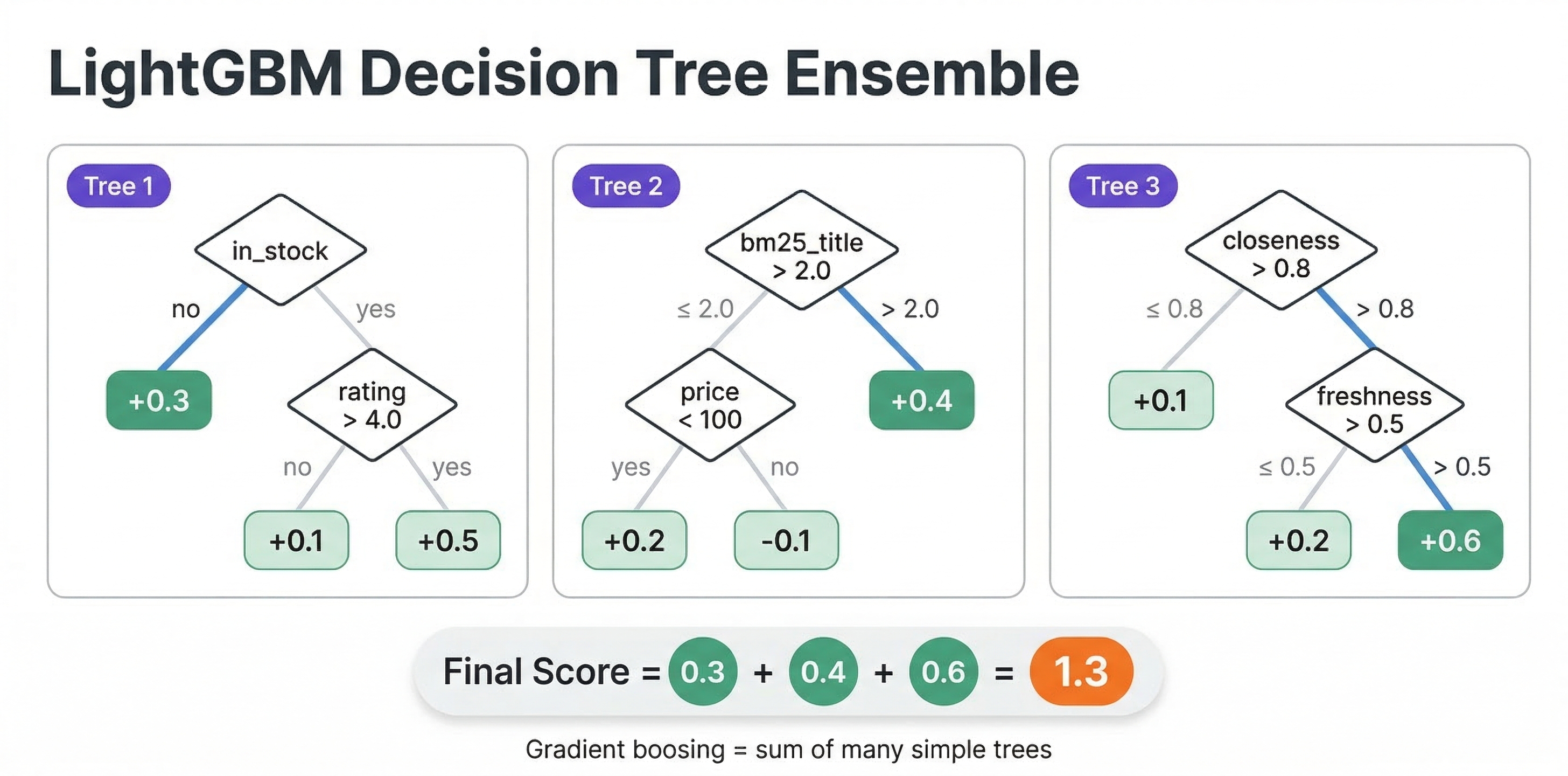
How Vespa evaluates GBDT models

An important detail: Vespa does not use the XGBoost or LightGBM libraries at runtime. Instead, it converts the exported model into its own optimized evaluation framework when you deploy the application. This means evaluation is fast and has no external dependencies. It also means the model format matters. Only the JSON export formats are supported because Vespa parses them into its internal representation.

The evaluation traverses the decision trees, resolving feature values from Vespa's rank feature system. Each tree produces a score, and the final score is the sum of all tree scores (standard gradient boosting). For classification models, you might want to wrap the output in a sigmoid() function:

second-phase {
    expression: sigmoid(xgboost("binary_classifier.json"))
}

Evaluating model quality

Before deploying a new model to production, you need to verify it actually improves ranking. There are two levels of evaluation: offline and online.

Offline evaluation

Offline evaluation uses a held-out test set of queries with relevance labels. You compute ranking metrics on this set and compare your new model against the baseline.

The most common metrics are:

NDCG@k (Normalized Discounted Cumulative Gain) measures ranking quality for graded relevance labels. It gives more credit to relevant documents appearing at higher positions. NDCG@10 evaluates the top 10 results and is the standard metric for web search and product search.

MRR (Mean Reciprocal Rank) measures how quickly the first relevant result appears. It is the average of 1/rank_of_first_relevant_result across queries. Good for navigational queries where the user wants one specific result.

MAP (Mean Average Precision) computes average precision at each relevant result position, then averages across queries. Works with binary relevance labels and is commonly used in information retrieval.

You can compute these with libraries like scikit-learn or dedicated LTR evaluation tools:

from sklearn.metrics import ndcg_score
import numpy as np

# For each query, compare model predictions against true labels
ndcg = ndcg_score([true_labels], [predicted_scores], k=10)
print(f"NDCG@10: {ndcg:.4f}")

Online evaluation with A/B testing

Offline metrics do not always predict online success. User behavior is complex, and lab conditions differ from production. A/B testing is essential for validating that a model change actually improves the user experience.

In Vespa, A/B testing is simple because you can have multiple rank profiles in the same schema:

rank-profile baseline {
    first-phase {
        expression: bm25(title) + bm25(body)
    }
}

rank-profile ltr_v2 {
    first-phase {
        expression: bm25(title) + bm25(body)
    }
    second-phase {
        expression: xgboost("ranker_v2.json")
        rerank-count: 200
    }
}

Your application routes users to different rank profiles:

# Control group
/search/?yql=...&ranking.profile=baseline

# Treatment group
/search/?yql=...&ranking.profile=ltr_v2

You can have ranker_v1.json and ranker_v2.json in the models/ directory simultaneously. Deploying a new model does not require re-indexing, just an application package redeployment. This makes it easy to iterate on models quickly.

Track online metrics like click-through rate, conversion rate, user engagement, and time to first click. Run the test long enough to reach statistical significance before drawing conclusions.

Iterating on your model

LTR is an iterative process. Your first model will likely use a handful of obvious features and produce modest improvements over the hand-tuned baseline. Over time, you add more features, collect more training data, tune hyperparameters, and the model gets better.

A typical iteration cycle looks like this:

1. Define a rank profile with summary-features or match-features to log features from your current ranking.
2. Collect queries, impressions, and clicks from production traffic.
3. Derive relevance labels from user behavior (covered in the training data chapter).
4. Train a model on the collected data.
5. Evaluate offline against a held-out test set.
6. Deploy and A/B test against the current model.
7. If the new model wins, promote it. Start the cycle again.

Each cycle produces a better model because you have more data, better features, and better understanding of what drives relevance for your specific use case.

Best practices

Start with a strong first-phase. Your LTR model typically runs in the second phase. The first phase determines which documents the model even gets to see. A weak first phase means the best documents might not make it to the second phase.

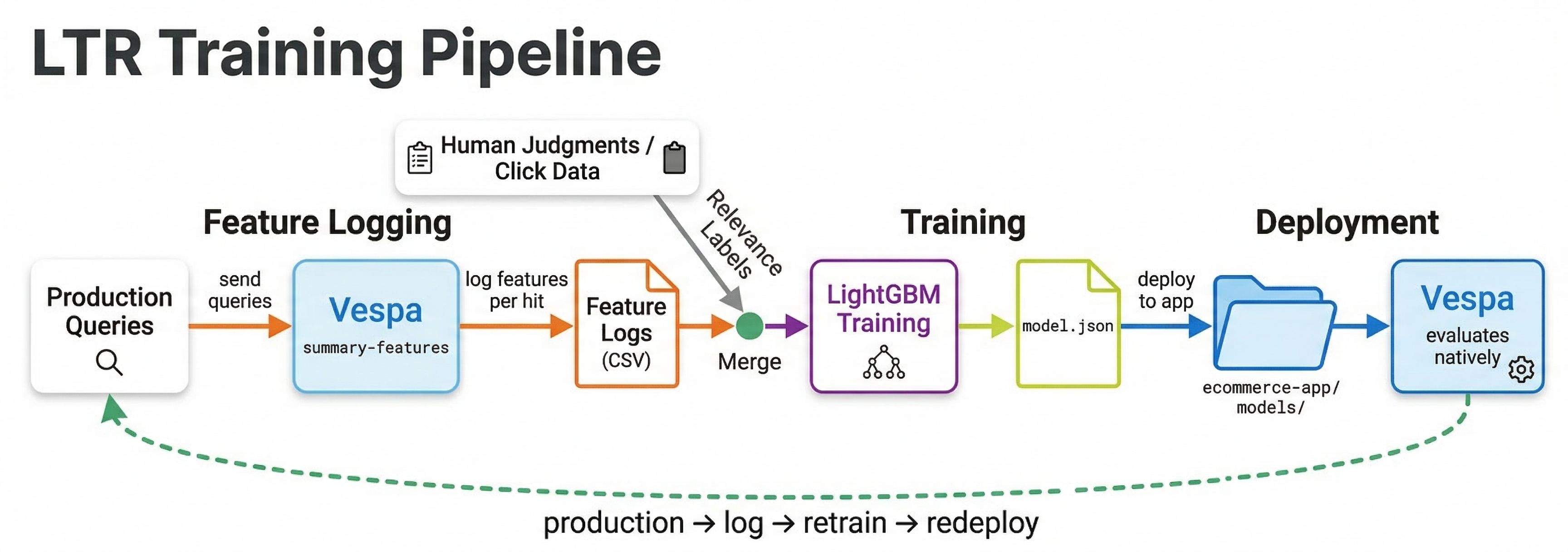
Train on features from Vespa. Always extract training features directly from Vespa using summary-features or match-features, not from offline recomputation. This prevents feature drift between training and serving. If BM25 is computed slightly differently offline than in Vespa, your model will underperform.

Keep models small for latency. A model with 500 trees of depth 8 evaluates much slower than one with 100 trees of depth 5. For second-phase ranking on 200 documents per content node, even moderately large models are fine. But if you ever use a model in first-phase, keep it very small.

Monitor feature distributions. Features can drift over time as content and queries change. A popularity feature that ranged 0-100 during training but now ranges 0-10000 will confuse the model. Regularly compare training feature distributions against production distributions.

Use early stopping during training. Train with a validation set and stop when the validation metric stops improving. This prevents overfitting and often produces smaller, faster models.

Next steps

You now know how to train XGBoost and LightGBM ranking models and deploy them in Vespa. In the next chapter, we explore neural re-rankers, specifically cross-encoder models that use deep learning for even more powerful re-ranking. These models are more expensive but can capture semantic understanding that GBDT models cannot.

For more details, see the Vespa XGBoost documentation, the LightGBM documentation, and the Vespa blog series on improving product search with LTR.