Neural re-rankers
In the previous chapter, we trained GBDT models like XGBoost and LightGBM for learning to rank. These models are fast and effective at combining hand-crafted features, but they have a limitation: they only work with features you explicitly define. They cannot discover new patterns in raw text. Neural re-rankers, specifically transformer-based models, can read the actual query and document text and learn deep semantic relationships that no hand-crafted feature can capture.
In this chapter, we explore how neural re-ranking works in Vespa. We cover the difference between bi-encoders and cross-encoders, how to deploy ONNX models for re-ranking, and how to set up a full cross-encoder pipeline. We also look at ColBERT as a middle ground between the two approaches.
Bi-encoders vs cross-encoders
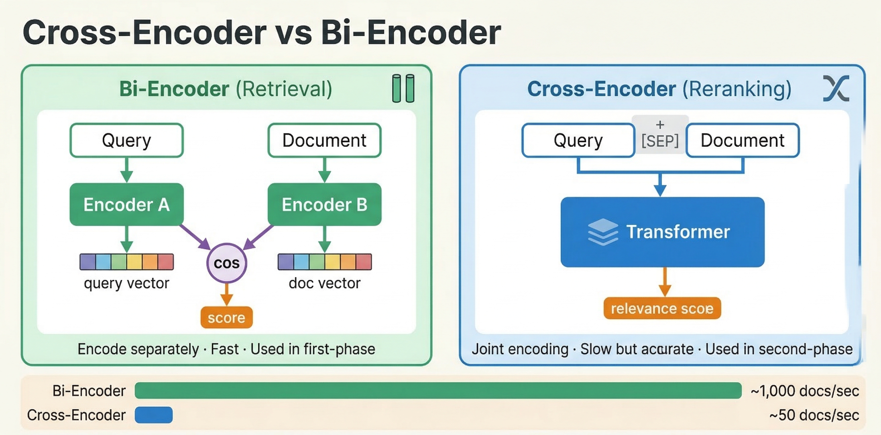
To understand neural re-ranking, you need to understand two fundamentally different architectures for scoring query-document pairs.
Bi-encoders
A bi-encoder processes the query and document independently. It encodes each into a separate vector embedding using a transformer model. Similarity is then computed using a simple operation like cosine similarity or dot product between the two vectors.
This is the approach we used in the vector search module. You embed your documents at indexing time and embed the query at search time, then use nearest neighbor search to find similar vectors. The key advantage is speed: document embeddings are computed once during indexing and reused for every query. Only the query needs to be embedded at search time.
The downside is that bi-encoders cannot capture fine-grained interactions between query and document tokens. Each text is compressed into a single fixed-size vector independently. The model never sees the query and document together, so it cannot reason about specific term relationships, negation, or contextual nuances.
Cross-encoders
A cross-encoder processes the query and document together as a single input. Both texts are concatenated and fed through a transformer model, which performs full cross-attention between every query token and every document token. The output is a single relevance score.
This joint processing makes cross-encoders significantly more accurate than bi-encoders. The model can attend to specific words in the query and see how they relate to specific words in the document. It can understand that "apple fruit nutrition" is about food, not computers, by looking at the document context.
The tradeoff is cost. A cross-encoder must run the full transformer forward pass for every query-document pair. You cannot pre-compute anything at indexing time. If you have 10,000 candidate documents, you need 10,000 forward passes per query. This is why cross-encoders are used strictly for re-ranking small candidate sets, not for initial retrieval.
The practical pattern
The standard approach in modern search systems is a multi-stage pipeline:
- Retrieve candidates using a fast method (BM25, bi-encoder ANN, or both)
- Re-rank the top candidates using a cross-encoder
In Vespa terms, retrieval happens during matching and first-phase ranking. Cross-encoder re-ranking happens in the global-phase, where you score a small set of globally merged top results.
ONNX models in Vespa
Vespa uses the ONNX Runtime for neural model inference. ONNX (Open Neural Network Exchange) is a standard format that most deep learning frameworks can export to. You train your model in PyTorch or TensorFlow, export it to ONNX format, and deploy it in Vespa.
Exporting a cross-encoder to ONNX
The easiest way to export a HuggingFace cross-encoder model is using the Optimum library:
pip install optimum[exporters]
optimum-cli export onnx --model cross-encoder/ms-marco-MiniLM-L-6-v2 model_output_dir/
This exports the model as model.onnx along with the tokenizer files. The ms-marco-MiniLM-L-6-v2 model is a popular choice for search re-ranking. It is small (about 22 million parameters) and fast, while still providing significant quality improvements over BM25.
You can also export programmatically:
from optimum.onnxruntime import ORTModelForSequenceClassification

model = ORTModelForSequenceClassification.from_pretrained(
    "cross-encoder/ms-marco-MiniLM-L-6-v2",
    export=True
)
model.save_pretrained("model_output_dir/")
For more control, use torch.onnx.export directly:
import torch
from transformers import AutoModelForSequenceClassification, AutoTokenizer

model_name = "cross-encoder/ms-marco-MiniLM-L-6-v2"
model = AutoModelForSequenceClassification.from_pretrained(model_name)
tokenizer = AutoTokenizer.from_pretrained(model_name)

dummy = tokenizer("query", "document", return_tensors="pt")
torch.onnx.export(
    model,
    (dummy["input_ids"], dummy["attention_mask"], dummy["token_type_ids"]),
    "model.onnx",
    input_names=["input_ids", "attention_mask", "token_type_ids"],
    output_names=["logits"],
    dynamic_axes={
        "input_ids": {0: "batch", 1: "sequence"},
        "attention_mask": {0: "batch", 1: "sequence"},
        "token_type_ids": {0: "batch", 1: "sequence"},
    }
)
The exported ONNX model must be self-contained (no external data files) and under 2GB.
Placing models in the application package
ONNX model files go in your application package, typically under models/:
myapp/
  models/
    cross-encoder.onnx
    tokenizer.json
  schemas/
    doc.sd
  services.xml
The tokenizer file is needed if you want Vespa to tokenize text at query time or indexing time. You configure it as a component in services.xml:
<container id="default" version="1.0">
    <component id="tokenizer" type="hugging-face-tokenizer">
        <model path="models/tokenizer.json"/>
    </component>
</container>
Setting up a cross-encoder in Vespa
A cross-encoder pipeline in Vespa involves three parts: storing document tokens, declaring the ONNX model in a rank profile, and wiring up the tokenization functions. Let's walk through each part.
Storing document tokens
Cross-encoders need tokenized input. Rather than tokenizing documents on every query (which would be very expensive), you tokenize them once at indexing time and store the token IDs as a tensor attribute.
In your schema, define a field for the pre-computed tokens:
field tokens type tensor<float>(d0[128]) {
    indexing: (input title || "") . " " . (input body || "") | embed tokenizer | attribute
}
This concatenates the title and body, runs the text through the tokenizer component, and stores the resulting token IDs as a dense tensor with up to 128 tokens. The dimension size (128 here) determines the maximum document length in tokens. Longer documents get truncated.
Declaring the ONNX model
In your rank profile, declare the ONNX model and map its inputs to Vespa functions:
rank-profile cross-encoder-reranker {
    inputs {
        query(q_tokens) tensor<float>(d0[32])
    }

    onnx-model cross_encoder {
        file: models/cross-encoder.onnx
        input input_ids: my_input_ids
        input attention_mask: my_attention_mask
        input token_type_ids: my_token_type_ids
    }

    function my_input_ids() {
        expression: tokenInputIds(256, query(q_tokens), attribute(tokens))
    }

    function my_token_type_ids() {
        expression: tokenTypeIds(256, query(q_tokens), attribute(tokens))
    }

    function my_attention_mask() {
        expression: tokenAttentionMask(256, query(q_tokens), attribute(tokens))
    }

    first-phase {
        expression: bm25(title) + bm25(body)
    }

    global-phase {
        rerank-count: 25
        expression: onnx(cross_encoder){d0:0,d1:0}
    }
}
Let's break down the key parts:
The onnx-model block declares the model file and maps its expected input names (input_ids, attention_mask, token_type_ids) to Vespa functions that produce the actual tensors.
The three tokenization functions use Vespa's built-in helpers:
tokenInputIds(max_length, query_tokens, doc_tokens)creates the concatenated token sequence with special tokens. It inserts[CLS]at the start,[SEP]between query and document, and[SEP]at the end, following the BERT input format.tokenTypeIds(max_length, query_tokens, doc_tokens)creates segment IDs: 0 for query tokens and 1 for document tokens. This tells the model which tokens belong to the query and which to the document.tokenAttentionMask(max_length, query_tokens, doc_tokens)creates the attention mask: 1 for real tokens and 0 for padding positions.
The first argument (256) is the maximum combined sequence length. This should be large enough to fit the query plus document tokens plus special tokens, but not so large that it wastes computation on padding. 256 tokens is a practical limit for most cross-encoder use cases.
The onnx(cross_encoder){d0:0,d1:0} expression evaluates the model and extracts the relevance score. The {d0:0,d1:0} part is tensor slicing to get a scalar from the model's output tensor.
Querying
At query time, you need to pass both the query embedding (for first-phase retrieval) and the tokenized query (for cross-encoder re-ranking):
{
    "yql": "select * from doc where {targetHits:200}nearestNeighbor(embedding, q)",
    "input.query(q)": "embed(e5, \"how does machine learning work\")",
    "input.query(q_tokens)": "embed(tokenizer, \"how does machine learning work\")",
    "ranking": "cross-encoder-reranker"
}
The embed(e5, ...) call generates the bi-encoder embedding for nearest neighbor retrieval. The embed(tokenizer, ...) call generates the token IDs for the cross-encoder. Both happen on the container node before the query is dispatched.
The pipeline then works as follows: nearest neighbor search retrieves the top 200 candidates using the bi-encoder embedding. First-phase ranking scores them with BM25. The results from all content nodes are merged. Global-phase re-ranks the top 25 merged results using the cross-encoder.
Non-BERT models
The built-in tokenization functions (tokenInputIds, tokenTypeIds, tokenAttentionMask) use BERT-style special token IDs (101 for [CLS], 102 for [SEP]). If you use a model with different tokenization conventions, like RoBERTa, use the custom variant:
function my_input_ids() {
    expression: customTokenInputIds(1, 2, 256, query(q_tokens), attribute(tokens))
}
The first two arguments are the start-of-sequence token ID and separator token ID for your specific model.
Quality vs latency tradeoffs
Cross-encoder re-ranking gives you better relevance at the cost of latency. The key parameters that control this tradeoff are the model size, sequence length, and rerank-count.
Model size
Smaller models are faster. The ms-marco-MiniLM-L-6-v2 model has 6 transformer layers and about 22 million parameters. It runs comfortably on CPU. Larger models like BERT-base (12 layers, 110M parameters) or DeBERTa-v3-large (24 layers, 300M+ parameters) produce better scores but are significantly slower.
For CPU inference, stick with small models like MiniLM variants. For larger models, use GPU acceleration.
Sequence length
Transformer complexity scales quadratically with input sequence length. A 256-token input is much faster than a 512-token input. For most search re-ranking, 256 tokens is sufficient since queries are typically short and you only need the most relevant portion of the document.
If your documents are long, consider storing tokens only from the title and first paragraph rather than the full body.
Rerank count
The rerank-count in global-phase directly determines how many cross-encoder evaluations happen per query. Re-ranking 25 documents is very different from re-ranking 200.
Practical guidelines from real benchmarks:
- Re-ranking 10-25 documents with a MiniLM model adds roughly 30-50ms to query latency on CPU.
- A full pipeline (query encoding + retrieval + re-ranking 25 docs) can run under 60ms end-to-end.
- Adding cross-encoder re-ranking can reduce throughput significantly (from thousands of QPS down to under 100 QPS), so size your infrastructure accordingly.
A three-stage pipeline is often practical for high-quality search: retrieve 1000 candidates with ANN, narrow to 100 with a second-phase GBDT model, then re-rank the top 25 with a cross-encoder in global-phase.
GPU acceleration
For larger models or higher rerank-counts, GPU acceleration makes a big difference. Configure it per model:
onnx-model cross_encoder {
    file: models/cross-encoder.onnx
    input input_ids: my_input_ids
    input attention_mask: my_attention_mask
    input token_type_ids: my_token_type_ids
    gpu-device: 0
}
The gpu-device: 0 parameter tells Vespa to use the first GPU. If no GPU is available, it falls back to CPU. On Vespa Cloud, you configure GPU resources through the cloud console. For local deployments, you need to expose NVIDIA GPUs to the Vespa container.
GPU becomes worthwhile for models exceeding roughly 30-40 million parameters, or when you need to re-rank more than 50 documents with any model.
ColBERT: late interaction models
Cross-encoders give the best quality but are expensive because they process query and document together at query time. Bi-encoders are fast because they pre-compute document embeddings but sacrifice quality because query and document never interact at the token level. ColBERT sits in between.
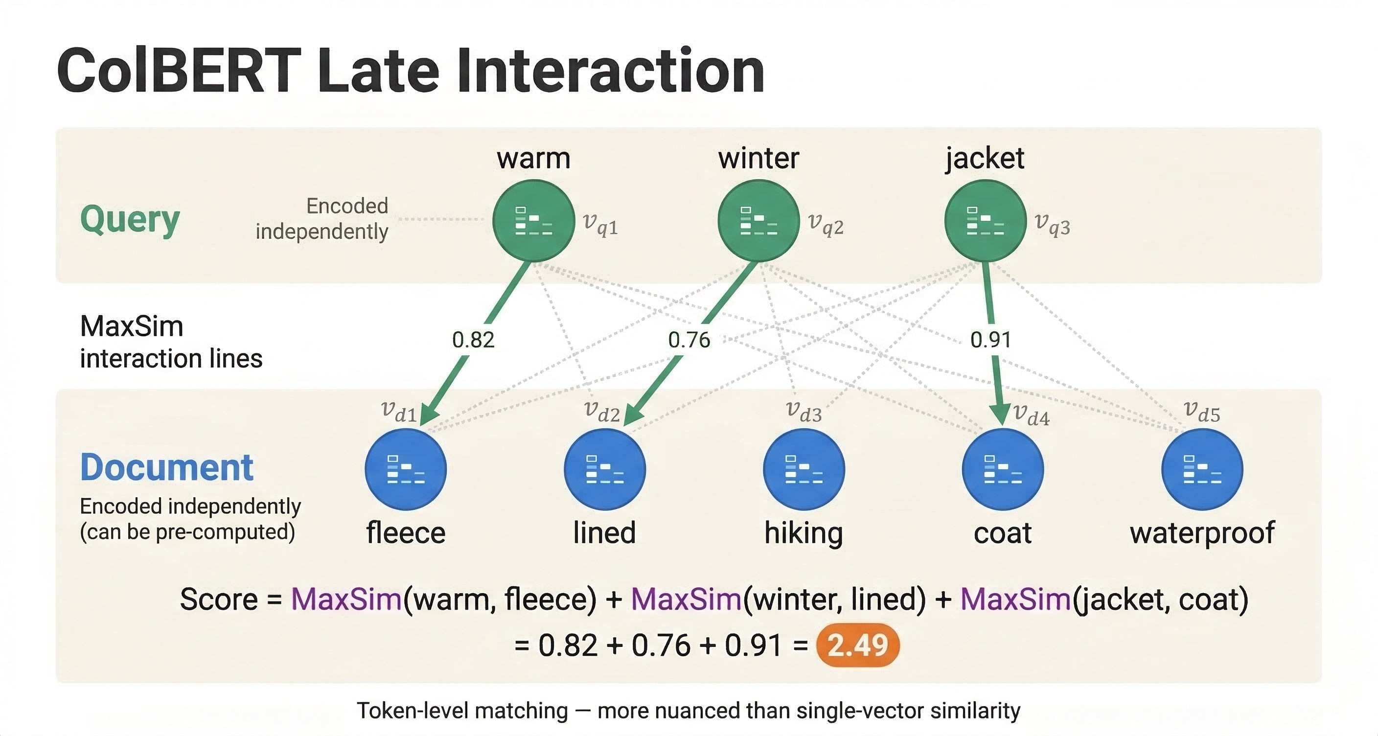
How ColBERT works
ColBERT (Contextualized Late Interaction over BERT) encodes query and document independently, like a bi-encoder, but instead of compressing each into a single vector, it keeps a vector for every token. A query with 10 tokens produces 10 vectors. A document with 100 tokens produces 100 vectors.
The similarity score is computed using MaxSim: for each query token vector, find the maximum similarity with any document token vector, then sum across all query tokens. This "late interaction" allows token-level matching while still enabling pre-computation of document token embeddings at indexing time.
The result is quality close to cross-encoders with much better performance, since document token embeddings only need to be computed once.
ColBERT in Vespa
Vespa has a built-in ColBERT embedder. Configure it in services.xml:
<container id="default" version="1.0">
    <component id="colbert" type="colbert-embedder">
        <transformer-model path="models/colbert-model.onnx"/>
        <tokenizer-model path="models/tokenizer.json"/>
    </component>
</container>
In your schema, define a multi-vector field for the token embeddings:
field colbert_tokens type tensor<float>(dt{}, x[128]) {
    indexing: input title . " " . input body | embed colbert | attribute
}
The dt{} is a mapped dimension where each key corresponds to a document token. The x[128] is the embedding dimension for each token vector.
For large-scale deployments, you can use binarized ColBERT with int8 quantization for a 32x storage reduction:
field colbert_tokens type tensor<int8>(dt{}, x[16]) {
    indexing: input title . " " . input body | embed colbert | attribute
}
ColBERT ranking expression
The MaxSim computation is expressed as a tensor operation in Vespa:
rank-profile colbert-ranking {
    inputs {
        query(qt) tensor<float>(qt{}, x[128])
    }

    first-phase {
        expression: bm25(title)
    }

    second-phase {
        rerank-count: 100
        expression {
            sum(
                reduce(
                    sum(query(qt) * attribute(colbert_tokens), x),
                    max, dt
                ),
                qt
            )
        }
    }
}
Reading the expression from inside out: sum(query(qt) * attribute(colbert_tokens), x) computes the dot product between each query token and each document token along the embedding dimension. reduce(..., max, dt) finds the maximum similarity document token for each query token. sum(..., qt) adds up the max similarities across all query tokens.
When to use ColBERT vs cross-encoders
ColBERT is a good choice when:
- You need better quality than bi-encoders but cannot afford cross-encoder latency for every query
- You can afford the extra storage for per-token embeddings (much more than a single vector per document)
- You want to re-rank a larger candidate set (100-200 documents) than is practical with cross-encoders
Cross-encoders are better when:
- You need the absolute highest quality re-ranking
- You only need to re-rank a small set (10-25 documents)
- You have GPU resources available
- Storage is more constrained than compute
In practice, you can even combine both: use ColBERT in the second-phase to re-rank 100 candidates, then use a cross-encoder in the global-phase to re-rank the top 25.
Stateless model evaluation
Beyond ranking, Vespa can evaluate ONNX models as a standalone service through its stateless model evaluation API. This is useful for tasks like classification, feature extraction, or any inference that does not need to be part of the ranking pipeline.
Add <model-evaluation/> to your services.xml:
<container id="default" version="1.0">
    <model-evaluation/>
</container>
Models placed in the models/ directory are automatically discovered and made available via a REST API at /model-evaluation/v1/. You can also call them from custom Java request handlers.
This is separate from ranking. For re-ranking, you always declare models in rank profiles as shown above. Stateless model evaluation is for other use cases where you need model inference as part of request processing.
A complete cross-encoder example
Let's put everything together in a complete working example. This shows a schema with both bi-encoder retrieval and cross-encoder re-ranking.
The schema:
schema doc {
    document doc {
        field title type string {
            indexing: summary | index
        }
        field body type string {
            indexing: summary | index
        }
    }

    field tokens type tensor<float>(d0[128]) {
        indexing: (input title || "") . " " . (input body || "") | embed tokenizer | attribute
    }

    field embedding type tensor<float>(x[384]) {
        indexing: input title . " " . input body | embed e5 | attribute | index
        attribute {
            distance-metric: angular
        }
        index {
            hnsw {
                max-links-per-node: 16
                neighbors-to-explore-at-insert: 200
            }
        }
    }

    rank-profile hybrid-with-cross-encoder {
        inputs {
            query(q) tensor<float>(x[384])
            query(q_tokens) tensor<float>(d0[32])
        }

        onnx-model cross_encoder {
            file: models/cross-encoder.onnx
            input input_ids: my_input_ids
            input attention_mask: my_attention_mask
            input token_type_ids: my_token_type_ids
        }

        function my_input_ids() {
            expression: tokenInputIds(256, query(q_tokens), attribute(tokens))
        }
        function my_token_type_ids() {
            expression: tokenTypeIds(256, query(q_tokens), attribute(tokens))
        }
        function my_attention_mask() {
            expression: tokenAttentionMask(256, query(q_tokens), attribute(tokens))
        }

        function text_score() {
            expression: bm25(title) * 2 + bm25(body)
        }

        function vector_score() {
            expression: closeness(field, embedding)
        }

        match-features: text_score vector_score

        first-phase {
            expression: text_score + vector_score * 10
        }

        global-phase {
            rerank-count: 25
            expression: onnx(cross_encoder){d0:0,d1:0}
        }
    }
}
The services.xml needs the embedder and tokenizer components:
<container id="default" version="1.0">
    <component id="e5" type="hugging-face-embedder">
        <transformer-model path="models/e5-small-v2.onnx"/>
        <tokenizer-model path="models/e5-tokenizer.json"/>
        <prepend>
            <query>query: </query>
            <document>passage: </document>
        </prepend>
    </component>
    <component id="tokenizer" type="hugging-face-tokenizer">
        <model path="models/tokenizer.json"/>
    </component>
</container>
And the query:
{
    "yql": "select * from doc where {targetHits:200}nearestNeighbor(embedding, q) or title contains 'machine learning'",
    "input.query(q)": "embed(e5, \"how does machine learning work\")",
    "input.query(q_tokens)": "embed(tokenizer, \"how does machine learning work\")",
    "ranking": "hybrid-with-cross-encoder"
}
This query retrieves candidates using both vector search and text matching. First-phase combines BM25 and vector similarity for a rough ranking. Global-phase re-ranks the top 25 merged results using the cross-encoder for maximum relevance.
Vespa Cloud vs local deployment
For neural re-rankers, the deployment environment matters more than for GBDT models, because neural models are compute-intensive.
On Vespa Cloud, you configure GPU resources through the console and deploy your application package as usual. The platform handles GPU provisioning and model loading. This is the easiest path for running large cross-encoder models.
For local deployment, you need to set up GPU passthrough to your Vespa container if you want GPU acceleration. Without GPU, stick with small models like MiniLM variants that run efficiently on CPU. Local deployment works fine for development and testing, but for production workloads with cross-encoders, GPU support is important.
Next steps
You now understand the landscape of neural re-ranking in Vespa. You know how cross-encoders differ from bi-encoders, how to deploy ONNX models, and how ColBERT provides a middle ground. In the next chapter, we cover performance and scaling considerations for ranking pipelines, including how to size your infrastructure and tune for latency.
For detailed documentation, see the Vespa cross-encoder guide, ONNX model documentation, and the ColBERT embedder guide.