Performance and scaling tips
Building a great ranking pipeline is only half the challenge. The other half is making it fast enough for production. A ranking expression that takes 500ms per query might produce beautiful results, but users will not wait around to see them. In this chapter, we cover how to measure, tune, and scale your Vespa ranking pipeline for production workloads.
This chapter focuses on practical performance tuning. We look at the cost of each ranking phase, how to store data efficiently for ranking, how to monitor and diagnose latency issues, and how to scale your Vespa deployment when you need more capacity.
Cost of each ranking phase
Each phase in the ranking pipeline has different performance characteristics. Understanding these costs helps you make informed decisions about what to compute where.
First-phase cost
First-phase ranking runs on every document that matches the query. If a query matches 100,000 documents, the first-phase expression runs 100,000 times on that content node. This is why first-phase must be cheap.
Simple expressions like bm25(title) + attribute(popularity) evaluate in nanoseconds per document. Even at 100,000 evaluations, that is under a millisecond. But add an expensive feature like fieldMatch(title) and the cost per document goes up significantly. fieldMatch analyzes term positions, proximity, and ordering, which takes microseconds rather than nanoseconds per document. At 100,000 evaluations, that could add hundreds of milliseconds.
The general rule: first-phase expressions should use only features that compute in nanoseconds. Stick to bm25(), nativeRank(), attribute(), freshness(), and simple arithmetic.
The keep-rank-count parameter (default 10,000) determines how many top-scoring documents survive first-phase. Reducing this saves memory but risks dropping relevant documents before they reach second-phase.
Second-phase cost
Second-phase runs on a small subset of first-phase results, controlled by rerank-count (default 100 per content node). With 100 evaluations, you can afford much more expensive expressions.
An XGBoost model with 200 trees of depth 5 evaluates in roughly 10-50 microseconds per document. At 100 documents, that is 1-5 milliseconds total. Even at rerank-count: 500, latency stays reasonable.
ONNX models in second-phase are trickier. A small model (under 10 million parameters) can handle hundreds of evaluations. But a large transformer model would be too slow for second-phase because it runs per document on each content node. Large models belong in global-phase where they only run on the final merged top results.
Global-phase cost
Global-phase runs on the container node after merging results from all content nodes. The rerank-count here applies to the globally merged set, not per node. So rerank-count: 100 means 100 evaluations total, regardless of how many content nodes you have.
The cost depends entirely on what you compute. Simple normalization functions like normalize_linear() or reciprocal_rank_fusion() are nearly free. A cross-encoder ONNX model scoring 25 documents adds 30-50ms on CPU. Scoring 100 documents with the same model might take 150-200ms.
For large ONNX models, GPU acceleration reduces global-phase latency dramatically. A model that takes 200ms on CPU might take 20ms on GPU.
Data transfer cost
An often overlooked cost is data transfer between content nodes and the container. When global-phase needs feature values, those values must be sent from content nodes to the container along with the search results.
If you declare a function as a match-feature, it gets computed on the content node and the scalar result is transferred. This is efficient. But if your global-phase tries to access raw tensors that were not pre-computed, Vespa needs to transfer the tensor data, which can be much larger.
Always pre-compute what the global-phase needs using match-features:
rank-profile efficient {
    function text_score() {
        expression: bm25(title) * 2 + bm25(body)
    }
    function vector_score() {
        expression: closeness(field, embedding)
    }

    match-features: text_score vector_score

    first-phase {
        expression: text_score + vector_score
    }

    global-phase {
        rerank-count: 100
        expression: normalize_linear(text_score) + normalize_linear(vector_score)
    }
}
The text_score and vector_score functions are computed on content nodes and transferred as scalar values. The global-phase then just normalizes these pre-computed values.
Efficient feature storage
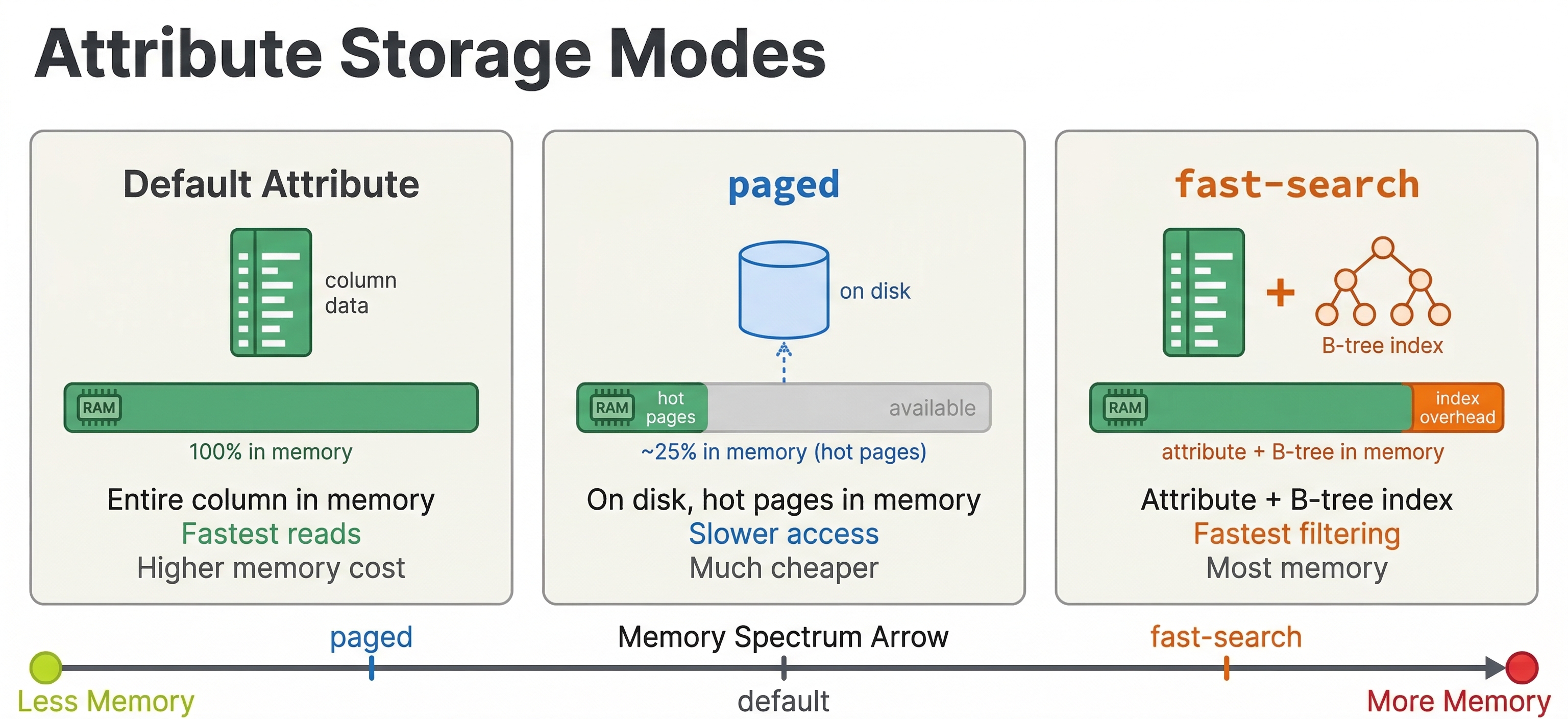
How you configure your schema fields affects ranking performance. The key settings are attribute storage modes and fast-search/fast-rank options.
Attributes for ranking
Any field used in ranking expressions must be stored as an attribute (in-memory). Fields used only for display in search results do not need to be attributes. This is an important distinction because attributes consume memory.
field popularity type int {
    indexing: summary | attribute
}

field full_description type string {
    indexing: summary | index
}
Here popularity is an attribute because it is used in ranking. full_description is indexed for text search but not an attribute because ranking does not directly access its raw value (BM25 uses the index, not the raw attribute).
fast-search and fast-rank
For attributes used in match-phase limiting, you need fast-search:
field popularity type int {
    indexing: summary | attribute
    attribute: fast-search
}
The fast-search option builds a B-tree index and a posting list for the attribute, enabling efficient filtering and match-phase limiting. It uses more memory but makes lookups faster.
For tensor attributes used in ranking expressions, fast-rank optimizes evaluation at the cost of higher memory usage:
field category_weights type tensor<float>(category{}) {
    indexing: attribute
    attribute: fast-rank
}
fast-rank is only supported for tensor types with at least one mapped dimension (sparse or mixed tensors). It stores the tensor in a layout that is more efficient for rank-expression evaluation, at the cost of extra memory.
Paged attributes
For attributes that are large but accessed infrequently (like in summary-features rather than first-phase), you can use paged attributes to reduce memory pressure:
field large_feature_vector type tensor<float>(x[1024]) {
    indexing: attribute
    attribute: paged
}
Paged attributes store data on disk with an in-memory cache. They work well for data accessed by second-phase or global-phase ranking (which only touch a small subset of documents) but are too slow for first-phase where every document is accessed.
One important warning: do not use paged on tensor fields that have HNSW indexing. The HNSW graph construction and search require random access to vector data, and paging that data to disk causes extremely poor performance during both feeding and querying.
HNSW index tuning
If your ranking pipeline includes nearest neighbor search, HNSW index parameters directly affect both recall and latency.
field embedding type tensor<float>(x[384]) {
    indexing: attribute | index
    attribute {
        distance-metric: angular
    }
    index {
        hnsw {
            max-links-per-node: 16
            neighbors-to-explore-at-insert: 200
        }
    }
}
max-links-per-node controls how many connections each node has in the HNSW graph. Higher values improve recall (finding the true nearest neighbors) at the cost of more memory and slower indexing. The default of 16 is a good starting point. Increase to 32 or 48 if recall is too low.
neighbors-to-explore-at-insert controls how many candidates are explored when inserting a new document into the graph. Higher values build a better graph at the cost of slower indexing. 200 is a reasonable default.
At query time, the targetHits parameter in the nearestNeighbor operator controls how many candidates the HNSW search explores. Higher values improve recall but increase latency:
{targetHits: 100}nearestNeighbor(embedding, query_embedding)
Start with targetHits equal to the number of results you need, then increase if recall is insufficient. You can also use hnsw.exploreAdditionalHits to search for more candidates than you return:
{targetHits: 100, hnsw.exploreAdditionalHits: 200}nearestNeighbor(embedding, query_embedding)
This searches for 300 candidates (100 + 200) but only returns the top 100 to ranking, improving recall without changing the number of documents that enter first-phase.
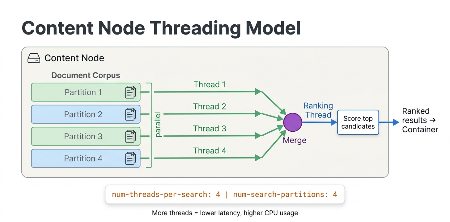
Threading and parallelism
Vespa can parallelize first-phase ranking across multiple threads on each content node:
rank-profile fast_first_phase {
    num-threads-per-search: 4
    min-hits-per-thread: 100

    first-phase {
        expression: bm25(title) + attribute(popularity)
    }
}
num-threads-per-search controls how many threads work on a single query's first-phase on one content node. The default is 1. Increasing this helps when first-phase needs to score many documents. With 4 threads, each thread scores a quarter of the matching documents.
min-hits-per-thread sets the minimum number of documents assigned to each thread. If a query matches 200 documents and min-hits-per-thread is 100, only 2 threads will be used even if num-threads-per-search is 4. This prevents the overhead of spawning threads when there is not enough work.
An important caveat: multi-threading helps most with linear operations like brute-force tensor evaluation and first-phase scoring over many documents. It does not help much with sublinear operators like WAND and approximate nearest neighbor (HNSW) search, because these operators already skip most documents. Adding threads to an HNSW search mostly adds overhead without reducing latency.
The num-threads-per-search setting in your rank profile controls per-query parallelism on each content node. The tradeoff is direct: more threads per query means fewer concurrent queries a node can handle. Choose based on whether your bottleneck is per-query latency (increase threads) or throughput (keep threads low).
Graceful degradation
When Vespa is under heavy load, queries might time out. Rather than returning errors, Vespa supports graceful degradation where partial results are returned within the time budget.
Soft timeout
By default, Vespa uses an adaptive timeout that tries to return results even if not all content nodes have finished. The coverage percentage in the response tells you how much of the corpus was searched.
You can configure timeout behavior per query:
/search/?yql=...&ranking.profile=my_profile&timeout=500ms
If the query takes longer than the timeout, Vespa returns whatever results have been collected so far, along with coverage information indicating how much of the data was searched.
For clusters with multiple content nodes, you can also configure adaptive coverage so that one slow node does not block the entire response:
<content id="search" version="1.0">
    <search>
        <coverage>
            <minimum>0.9</minimum>
            <min-wait-after-coverage-factor>0.2</min-wait-after-coverage-factor>
            <max-wait-after-coverage-factor>0.3</max-wait-after-coverage-factor>
        </coverage>
    </search>
</content>
With this configuration, once 90% of nodes have responded, Vespa starts a short additional wait period and then returns results. This prevents a single slow node from adding hundreds of milliseconds to every query. The response includes a coverage object that tells you what fraction of the data was actually searched, so your application can decide whether to show a warning to the user.
Rank-score-drop-limit
Use rank-score-drop-limit in first-phase to aggressively drop low-scoring documents:
first-phase {
    expression: bm25(title)
    rank-score-drop-limit: 0.5
}
Documents scoring 0.5 or below are dropped immediately, reducing the work for subsequent phases. Be careful with the threshold. Set it too high and you drop relevant documents. Set it too low and it has no effect.
Match-phase limiting
As discussed in the multi-phase ranking chapter, match-phase limiting caps the number of documents entering first-phase. This is the most powerful knob for reducing latency on broad queries:
rank-profile with_limiting {
    match-phase {
        attribute: popularity
        order: descending
        max-hits: 10000
    }
    first-phase {
        expression: bm25(title) + attribute(popularity) * 0.1
    }
}
Remember that match-phase limiting can backfire with restrictive filters. Monitor the content.proton.documentdb.matching.rank_profile.limited_queries metric to understand its impact.
Monitoring ranking latency
You cannot optimize what you do not measure. Vespa exposes detailed metrics for ranking performance.
Key metrics
Query latency metrics are available through the Vespa metrics API at /metrics/v2/values:
query_latency- total query latency including networkcontent.proton.documentdb.matching.rank_profile.query_latency- matching and ranking latency per rank profilecontent.proton.documentdb.matching.docs_matched- number of documents matched per querycontent.proton.documentdb.matching.docs_reranked- number of documents that entered second-phase
Additional useful metrics:
content.proton.documentdb.matching.rank_profile.rerank_time- time spent specifically on second-phase rankingcontent.proton.documentdb.matching.soft_doomed_queries- queries that hit the soft timeout and returned partial resultscontent.proton.executor.match.utilization- how saturated the match executor is (when sustained near 1.0, all query slots are busy and you need more capacity)
These metrics help you identify bottlenecks. If docs_matched is very high, your queries are too broad and match-phase limiting or better query filters would help. If docs_reranked is close to rerank-count, you are using all the second-phase budget and might benefit from increasing it or improving first-phase quality. If soft_doomed_queries is increasing, your queries are running too close to timeout and you need to either simplify ranking or add capacity.
Benchmarking with vespa-fbench
For systematic load testing, use vespa-fbench:
vespa-fbench -n 10 -q queries.txt -c 0 -o output.txt localhost 8080
This sends queries from queries.txt using 10 concurrent clients and reports latency percentiles. Run benchmarks before and after ranking changes to quantify their impact.
The query file format is one query URL per line:
/search/?yql=select%20*%20from%20doc%20where%20title%20contains%20%22laptop%22&ranking=my_profile
/search/?yql=select%20*%20from%20doc%20where%20title%20contains%20%22phone%22&ranking=my_profile
Scaling content and container nodes
When tuning is not enough, you need more hardware. Vespa scales differently for content and container nodes.
When to add content nodes
Content nodes hold data and run first-phase and second-phase ranking. Add more content nodes when:
- First-phase latency is too high because each node has too many documents to score. More nodes means each node holds fewer documents, reducing per-node matching and first-phase work.
- Memory is full because attributes and indexes exceed available RAM. More nodes spread the data across more machines.
- Second-phase is a bottleneck because complex models take too long on a single node's worth of candidates.
With flat distribution (the default), documents are spread evenly across all content nodes. Adding a node from 3 to 4 reduces each node's document count by 25%.
When to add container nodes
Container nodes are stateless and handle query parsing, dispatching to content nodes, merging results, and global-phase ranking. Add more container nodes when:
- Global-phase is expensive because cross-encoder models or complex ONNX inference dominate latency. Container nodes do not share global-phase work, so more containers serve more concurrent queries.
- Query throughput is the bottleneck rather than per-query latency. Each container can handle some number of concurrent queries. More containers means more concurrent capacity.
- Embedding computation is slow because query-time embedding (calling
embed()functions) runs on containers.
Container nodes are easy to add because they are stateless. No data redistribution is needed. Just start more instances and the load balancer distributes queries.
Grouped distribution
For high-availability and certain performance scenarios, Vespa supports grouped distribution where data is replicated across groups of content nodes:
<content id="search" version="1.0">
    <redundancy>2</redundancy>
    <group>
        <distribution partitions="1|*"/>
        <group distribution-key="0" name="group0">
            <node distribution-key="0" hostalias="node0"/>
            <node distribution-key="1" hostalias="node1"/>
        </group>
        <group distribution-key="1" name="group1">
            <node distribution-key="2" hostalias="node2"/>
            <node distribution-key="3" hostalias="node3"/>
        </group>
    </group>
</content>
With grouped distribution, each group holds a complete copy of the data. A query only needs to hit one group. This reduces the number of content nodes involved per query (fewer network round trips) and provides redundancy. If one group goes down, the other continues serving.
Grouped distribution is particularly beneficial when second-phase or first-phase latency is dominated by the slowest content node (tail latency). With fewer nodes per group, there is less chance of one slow node delaying the entire query.
Practical optimization checklist
Here is a checklist for optimizing a ranking pipeline, roughly in order of impact:
-
Profile your queries. Use the metrics API to find where time is spent. Is it matching, first-phase, second-phase, or global-phase? Optimize the bottleneck, not everything.
-
Reduce documents matched. Better query filters, match-phase limiting, or
rank-score-drop-limitreduce the workload for all subsequent phases. -
Keep first-phase cheap. Replace
fieldMatch()withbm25()if first-phase is too slow. Move expensive features to second-phase. -
Right-size rerank-count. Start with the minimum that gives acceptable quality. 50-100 for second-phase, 25-50 for global-phase with neural models.
-
Pre-compute for global-phase. Use match-features to avoid transferring raw data to the container.
-
Use appropriate attribute modes.
fast-searchfor match-phase attributes,fast-rankfor tensors used in ranking,pagedfor large attributes only needed in second-phase. -
Tune HNSW for your recall needs. Do not over-provision
targetHitsif lower values give acceptable recall. -
Parallelize first-phase. Increase
num-threads-per-searchif first-phase scores many documents. -
Scale horizontally. Add content nodes for data/ranking bottlenecks, container nodes for throughput/global-phase bottlenecks.
-
Consider GPU for global-phase. If cross-encoder models dominate latency, GPU can provide a 5-10x speedup.
Vespa Cloud vs local deployment
Performance tuning differs slightly between local and cloud deployments.
On Vespa Cloud, you configure node counts and resource allocation through the deployment specification. The platform handles node provisioning, and you can easily experiment with different configurations. GPU resources for global-phase are available through the cloud console.
For local deployment, you manage hardware directly. Use Docker for development and testing. For production, deploy on bare metal or VMs with sufficient memory for your attributes and indexes. GPU setup requires NVIDIA container toolkit configuration.
In both cases, the ranking configuration and tuning parameters are identical. The difference is operational: how you provision and manage the infrastructure.
Next steps
You now have a practical toolkit for making ranking pipelines fast. You know how to measure latency, identify bottlenecks, and apply the right optimizations. In the next chapter, we cover how to generate and use training data for learning-to-rank models, closing the loop on the full LTR workflow.
For comprehensive performance guidance, see the Vespa practical search performance guide and the sizing guide.