Approximate Nearest Neighbor Search

In the previous chapter, you learned how to store vector embeddings in Vespa using tensors. Now let's go deeper into how that search actually works with vectors. We have seen examples of nearestNeighbor in YQL. When we call nearestNeighbor, Vespa doesn't just compare the query vector against every single document vector. That would be too slow for any real world dataset. Instead, Vespa uses ANN (approximate nearest neighbor) search. The ANN algorithm Vespa uses is called HNSW, and it finds similar vectors quickly. Since it's "approximate", there is always a small tradeoff in accuracy, but for a massive gain in speed.

This chapter covers how the HNSW algorithm works, what distance metrics mean in practice, how to tune the index for your use case, and some important behaviors around filtering.

The Nearest Neighbor Problem

The core idea is simple. You have a query vector and a bunch of document vectors, and you want to find the documents whose vectors are closest to the query. "Closest" is defined by the distance metric you're using.

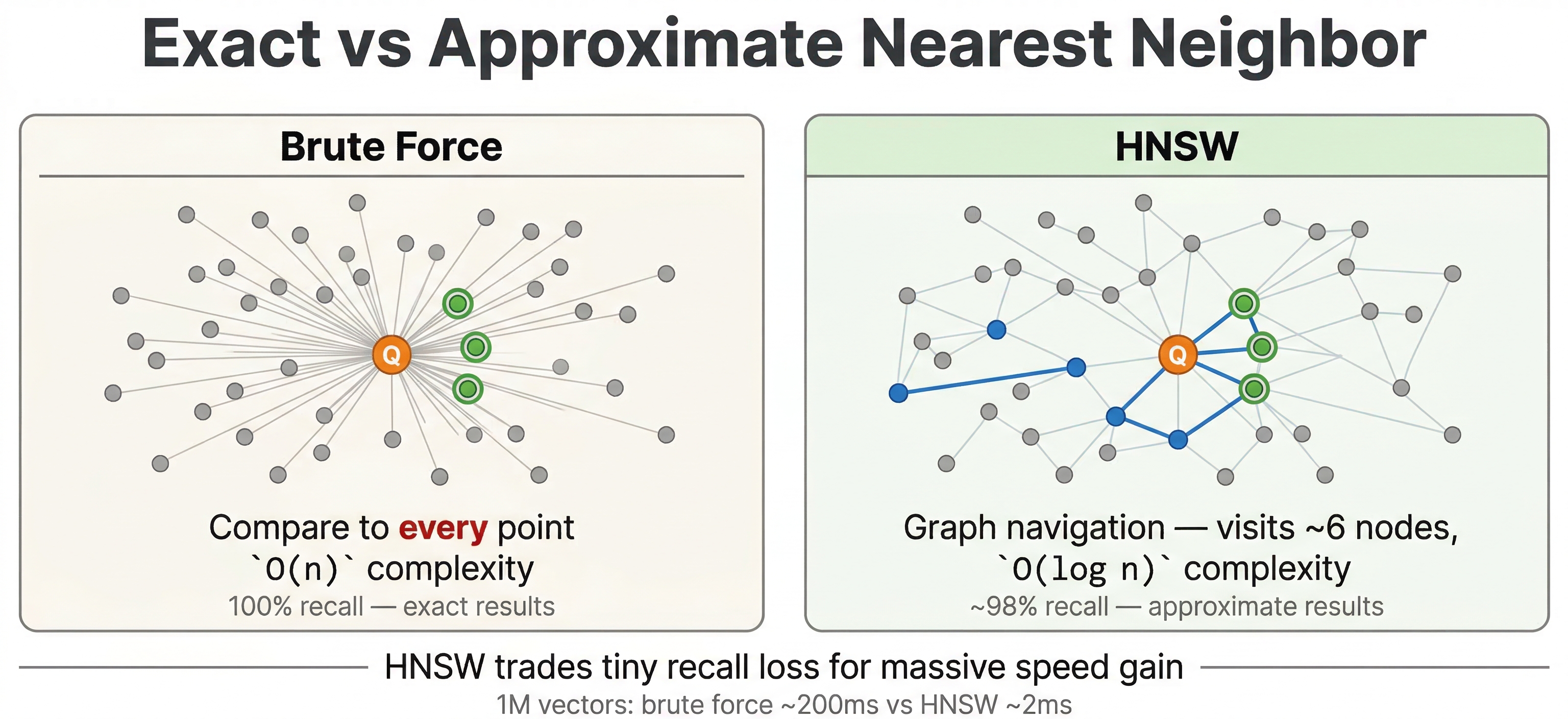
For a small dataset, you could just compute the distance from the query to every document, sort the results, and return the top ones. This is called exact nearest neighbor search, and it gives you perfect results. The problem is that it scales linearly. If you have millions of documents, you're doing millions of distance computations per query. At a billion documents, it's a billion computations. That's not going to work when you need responses in milliseconds and you need responses in milliseconds.

Approximate nearest neighbor search solves this by building an index structure that lets you quickly jump to the right neighborhood in vector space without checking each and every vector. The results you get back are very close to true nearest neighbors, and the search is orders of magnitude faster. For most applications, the tiny accuracy tradeoff is almost always well worth it.

What is HNSW?

Vespa uses HNSW (Hierarchical Navigable Small World) for approximate nearest neighbor search. It's one of the most popular ANN algorithms because it offers a great balance of speed, accuracy, and support for real-time updates.

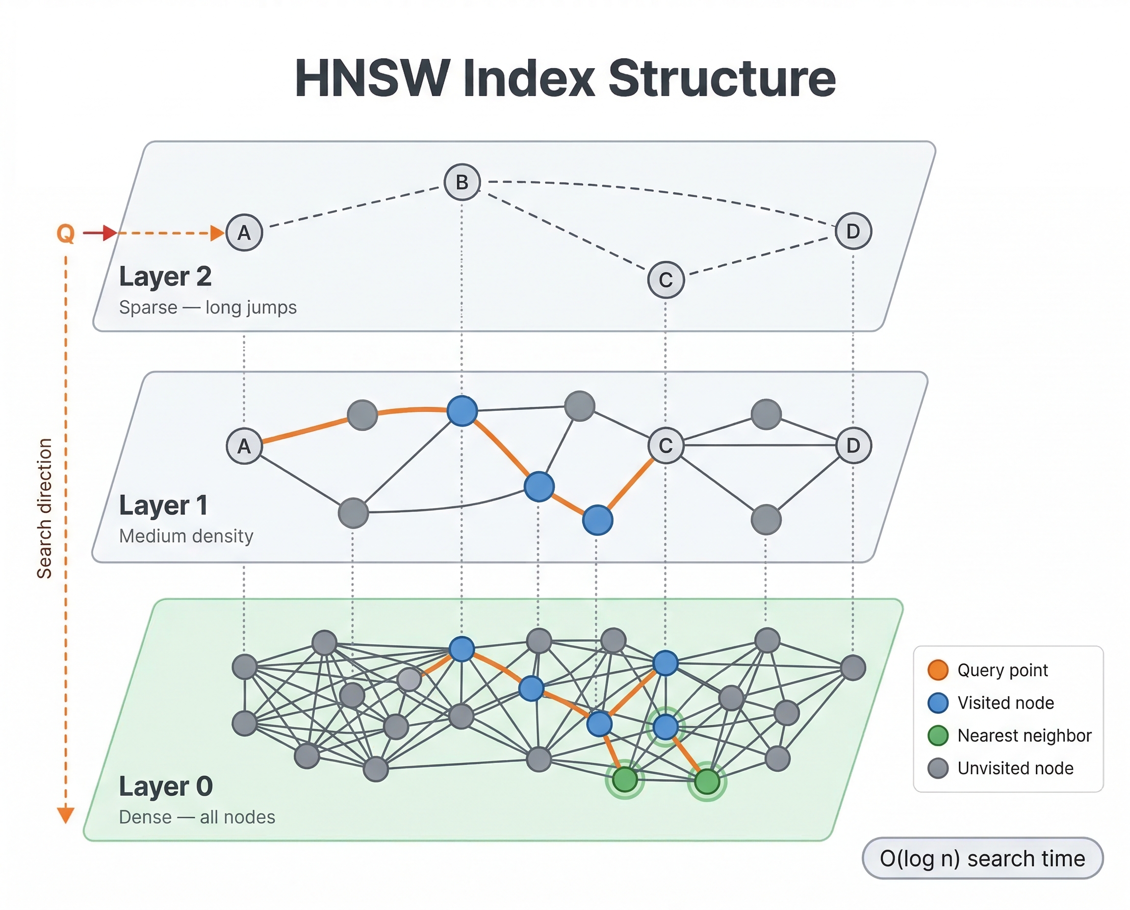
The basic idea is that HNSW builds a graph where each vector is a node, and edges connect vectors that are similar to each other. To find nearest neighbors, you start at some entry point in the graph and greedily walk toward your query vector, always moving to whichever neighbor is closer to the query. Because the graph connects similar vectors, this greedy walk quickly gets you to the right neighborhood.

What makes HNSW special is the "hierarchical" part. The graph has multiple layers. The top layers are sparse, with only a few nodes and long-range connections. As you go down, layers get denser with more nodes and shorter-range connections. The bottom layer contains every vector.

When a query comes in, here's what happens:

1. Start at a fixed entry point on the top layer
2. Greedily navigate to the closest node on that layer
3. Drop down to the next layer and continue navigating from there
4. Repeat until you reach the bottom layer
5. Do a more thorough local search on the bottom layer to find the actual nearest neighbors

The top layers let the algorithm make big jumps across vector space quickly, like taking a highway. The bottom layers handle the fine-grained local search, like navigating side streets. This hierarchy is what makes HNSW both fast and accurate.

When new documents are fed to Vespa, their vectors get inserted into the HNSW graph in real time. The algorithm finds the right place for the new vector and connects it to its nearest neighbors in the graph. This means new documents are searchable immediately after feeding, with no batch reindexing needed.

Distance Metrics

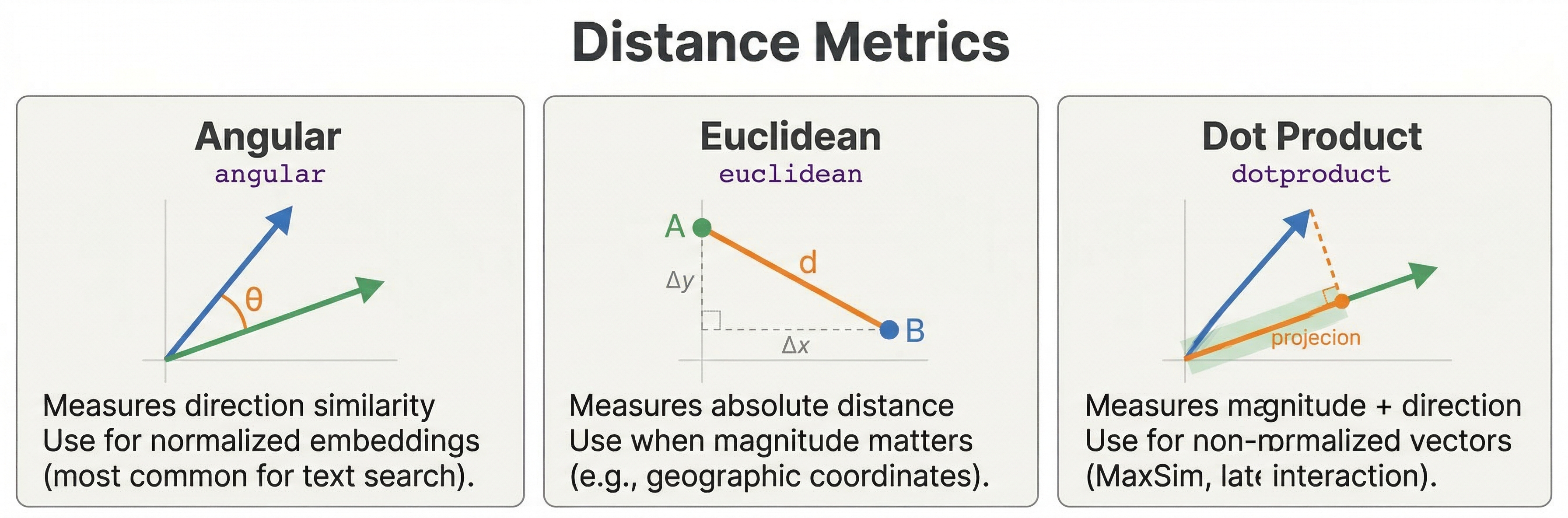
In the previous chapter, you saw that you configure a distance metric in your schema when defining a tensor field. Let's look at what each metric actually means and when to use it.

• Angular distance measures the angle between two vectors, ignoring their magnitude. It is the most common choice for text embeddings. Two vectors pointing in the same direction have zero angular distance, even if one is much longer than the other. This is what you want for most language model embeddings because the direction of the vector captures semantic meaning, not the length.

• Euclidean distance measures the straight-line distance between two points in vector space. Unlike angular distance, magnitude matters here. Two vectors can point in the same direction but have large Euclidean distance if one is much longer. Some image embeddings and specialized models work better with Euclidean distance, so check your model's documentation.

• Dot product computes the inner product of two vectors. For normalized vectors (unit length), dot product gives the same ranking as angular distance. But for unnormalized vectors, it lets magnitude influence similarity. One thing to watch out for: dot product isn't a true distance metric. Larger values mean more similar, which is the opposite of distances where smaller is better. Vespa handles this internally so that closeness() still returns higher values for more similar documents.

• Prenormalized-angular gives the same ordering as angular distance but is more efficient when your vectors are already normalized to unit length. If your embedding model produces normalized vectors (many do), this is a good optimization.

• Hamming distance counts the number of differing bits between binary vectors. This is a specialized metric used with binary quantized embeddings where each dimension is reduced to a single bit. You won't need this unless you're doing binary quantization.

For most text search applications, go with angular. If your model outputs normalized vectors, prenormalized-angular is faster. If you're unsure, check your embedding model's documentation for what it recommends.

targetHits

When you write a query like this:

select * from doc where {targetHits: 10}nearestNeighbor(embedding, query_embedding)

The targetHits: 10 parameter is a hint to the HNSW algorithm indicating how many neighbors to consider during graph traversal. It's not a limit on how many results you get back. The actual number of results returned is controlled by the hits query parameter (default 10) or the limit clause in YQL.

If you set targetHits: 10 but hits=5, Vespa finds approximately 10 nearest neighbors during the HNSW search, then returns the top 5 after ranking. If you set targetHits: 10 but hits=20, you might get fewer than 20 results because the HNSW search only looked for 10 candidates.

As a rule of thumb, set targetHits to at least the number of results you want to return. If you're using second-phase ranking or filters, you might want targetHits to be higher than your final result count so the later stages have enough candidates to work with.

Scoring Results: closeness() and distance()

Finding nearest neighbors is only half the story. You also need to score the results so Vespa can rank them. This is where closeness() and distance() come in.

The closeness(field, embedding) rank feature returns a value between 0 and 1, where 1 means the vectors are identical and 0 means they're maximally different. This works the same way regardless of which distance metric you configured. Whether you're using angular, euclidean, or dot product, closeness always gives you higher values for more similar documents. This makes it easy to combine with other scoring signals in rank profiles.

The distance(field, embedding) rank feature returns the raw distance value. The scale depends on your distance metric. For angular distance, it ranges from 0 to pi (approximately 3.14). For euclidean distance, it can be any non-negative number. Lower values mean more similar.

For most ranking expressions, you'll want closeness() because it's normalized and "higher is better" plays nicely with other signals like BM25 scores:

rank-profile semantic {
    inputs {
        query(query_embedding) tensor<float>(x[384])
    }
    first-phase {
        expression: closeness(field, embedding)
    }
}

If you need more control, you can use distance() and apply your own transformation. But closeness() is the right choice in most cases.

HNSW Index Tuning

The HNSW index has two main configuration parameters that control the tradeoff between search quality, memory usage, and indexing speed. You set these in your schema:

field embedding type tensor<float>(x[384]) {
    indexing: attribute | index
    attribute {
        distance-metric: angular
    }
    index {
        hnsw {
            max-links-per-node: 16
            neighbors-to-explore-at-insert: 200
        }
    }
}

• max-links-per-node controls how many edges each node has in the HNSW graph. More links means more paths to reach any given vector, which improves search quality. But more links also means more memory and slower index building. The default is 16, and values between 16 and 32 work well for most datasets. Going above 32 rarely helps and costs a lot of extra memory.

• neighbors-to-explore-at-insert controls how thoroughly the algorithm searches the graph when inserting a new vector. Higher values produce a better-connected graph (which means better search quality) at the cost of slower feeding. The default is 200. If you're seeing poor recall in your search results, try increasing this to 400 or 500. If feeding is too slow and you can accept slightly lower quality, you can decrease it.

For most applications, the defaults are fine. Only change these if you've measured a problem. If your search quality is good but feeding is slow, lower neighbors-to-explore-at-insert. If search quality is poor, increase max-links-per-node or neighbors-to-explore-at-insert.

Query-Time Tuning

Beyond index configuration, you can turn a few knobs at query time to control search behavior.

The approximate Parameter

By default, nearestNeighbor uses the HNSW index for fast approximate search. You can force exact search by setting approximate: false:

select * from doc where {targetHits: 10, approximate: false}nearestNeighbor(embedding, query_embedding)

With exact search, Vespa computes the distance to every single vector and returns the true nearest neighbors. This is slow but gives perfect results. Use it for small datasets, debugging, or when you need guaranteed accuracy. For production queries on any dataset of meaningful size, stick with the default approximate: true.

hnsw.exploreAdditionalHits

This is an important query-time parameter that many people miss. It tells the HNSW algorithm to explore more nodes than targetHits during the graph traversal:

vespa query \
  "yql=select * from doc where {targetHits: 10}nearestNeighbor(embedding, query_embedding)" \
  "input.query(query_embedding)=[0.1, 0.2, ...]" \
  "ranking.matching.numThreadsPerSearch=1" \
  "hnsw.exploreAdditionalHits=100"

With targetHits: 10 and hnsw.exploreAdditionalHits: 100, the algorithm explores 110 nodes total during the graph search. This improves recall (the chance of finding the true nearest neighbors) at the cost of slightly higher latency. If you're combining ANN with filters, increasing this value is especially important because some of the explored nodes might get filtered out.

Automatic Fallback to Exact Search

Here's something good to know: when you combine ANN search with a very restrictive filter and Vespa estimates that very few documents match the filter, it may automatically fall back to exact nearest neighbor search on just those matching documents. This is actually faster than navigating the HNSW graph when only a tiny fraction of documents pass the filter.

You don't need to configure this. Vespa makes the decision automatically based on the estimated filter selectivity. But it's useful to understand this behavior because you might notice that certain filtered queries are slower or faster than you expected.

Filtering with ANN Search

One of Vespa's strengths is combining nearest neighbor search with filters in a single query:

select * from doc where {targetHits: 10}nearestNeighbor(embedding, query_embedding) and category = "technology"

This finds the nearest neighbors among documents in the "technology" category. You can use any filter conditions you'd normally use in Vespa: date ranges, category matches, boolean flags, numeric ranges, or complex combinations with and/or.

Pre-filtering vs Post-filtering

How Vespa handles the filter internally depends on how selective it is. There are two strategies:

• Pre-filtering means Vespa applies the filter first and then searches only the matching vectors. If your filter matches a large portion of the data (say, 20% or more), this is efficient because the HNSW graph is still well-connected among the matching documents.

• Post-filtering means Vespa runs the ANN search first to find candidate vectors, then removes candidates that don't pass the filter. This can happen when the filter is moderately selective and pre-filtering would be too expensive.

Vespa chooses between these strategies automatically. You don't need to configure it. But there's an important practical implication: if your filter is very restrictive and eliminates most of the ANN candidates, you might get fewer results than you asked for. For example, if targetHits: 10 finds 10 neighbors but only 3 pass the filter, you get 3 results.

The fix is to increase targetHits or use hnsw.exploreAdditionalHits to give the algorithm more candidates before filtering. If your filters are highly selective, you should increase these values to compensate:

select * from doc where {targetHits: 100}nearestNeighbor(embedding, query_embedding) and rare_category = "niche_topic"

For more details on how Vespa optimizes filtered ANN search, see the nearest neighbor search guide.

Performance Characteristics

HNSW search time grows logarithmically with the number of vectors. Searching 1 million vectors takes only slightly longer than searching 100,000. This logarithmic scaling is what makes HNSW practical for very large datasets.

Memory usage is proportional to the number of vectors times the vector dimensions, plus the HNSW graph overhead. A rough rule of thumb is to budget 2-3x the raw embedding size. For a tensor<float>(x[384]) field (about 1.5 KB per document), expect around 3-4.5 KB per document total with the index. For a million documents, that's 3-4.5 GB for the embedding field.

Feeding throughput depends on neighbors-to-explore-at-insert. With default settings, Vespa can handle thousands of vector inserts per second per node. Documents become searchable immediately after feeding with no batch reindexing needed. This real-time indexing is a significant advantage over systems that require periodic index rebuilds.

Best Practices

• Start with default HNSW parameters (max-links-per-node: 16, neighbors-to-explore-at-insert: 200). Only tune if you've measured a quality or performance problem.

• Set targetHits to at least the number of results you want back. If you're using filters or second-phase ranking, set it higher to give those stages enough candidates.

• Use hnsw.exploreAdditionalHits when combining ANN with restrictive filters. This gives the algorithm more room to find neighbors that also pass the filter.

• Use closeness(field, embedding) in your rank profiles rather than distance(). It's normalized, always between 0 and 1, and "higher is better" makes it easy to combine with other signals.

• Monitor recall if accuracy matters for your application. Compare ANN results against exact search (approximate: false) on a sample of queries to verify that the approximate results are good enough.

• Keep targetHits reasonable. Asking for 10 neighbors is much faster than asking for 1000. Only request what you actually need.

Next Steps

You now understand how ANN search works in Vespa, from the HNSW algorithm to distance metrics to query-time tuning. The next chapter explores hybrid search, where you combine vector search with traditional text search to get the best of both worlds.

For detailed reference, see the nearest neighbor search guide and the nearestNeighbor YQL reference.