Grouping and Aggregations

Beyond returning ranked documents, search applications often need to provide facets, counts, histograms, and aggregated statistics. E-commerce sites show category counts and price ranges. News sites group articles by topic. Analytics dashboards compute sums and averages. Vespa's grouping language handles all these use cases. In this chapter, we explore how to group results and compute aggregations.

What is Grouping

Grouping takes a set of query results and organizes them into buckets based on field values. For each bucket, you can compute aggregations like counts, sums, averages, or return sample documents. The grouping language describes these operations in a declarative way.

Grouping queries are added to your YQL after a pipe symbol:

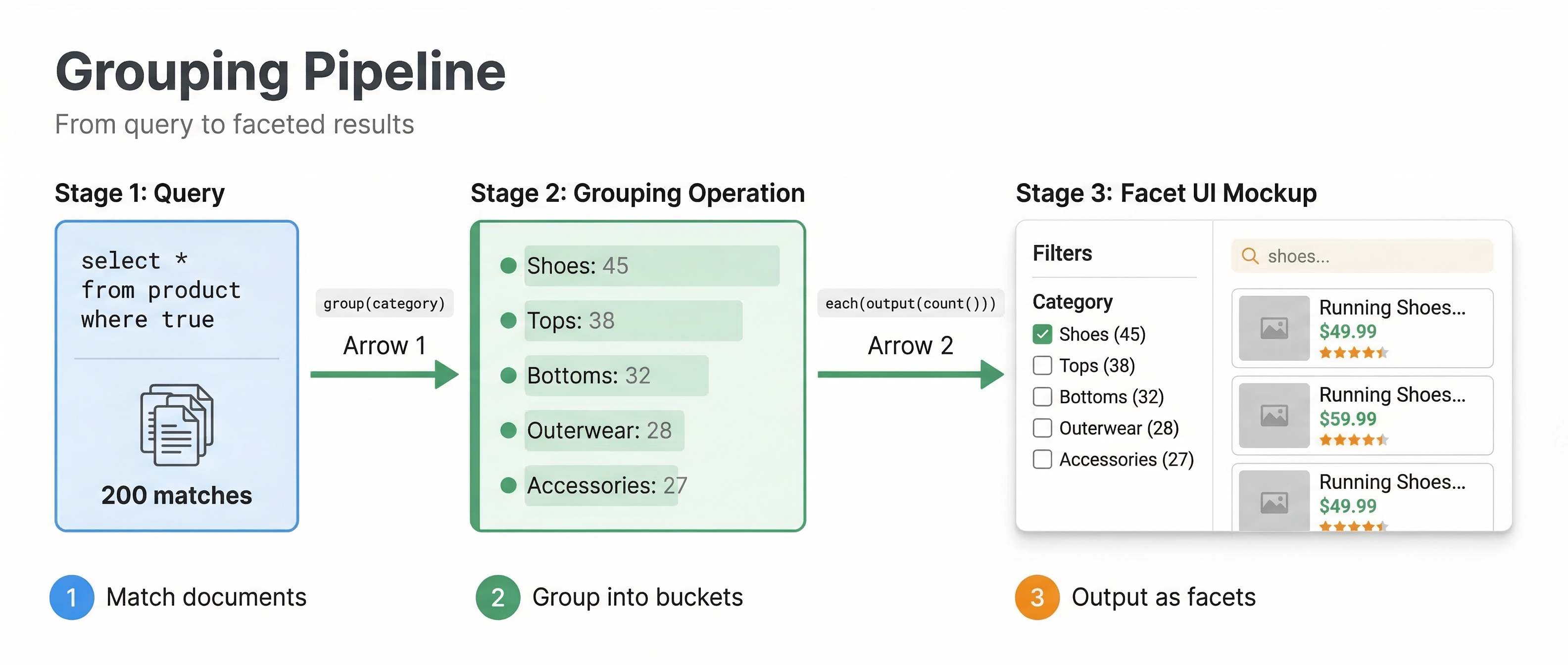
select * from product where title contains "laptop" | all(group(category) each(output(count())))

This query searches for laptops and groups results by category, outputting the count in each category. The result includes facet data showing how many laptops exist in each category.

Basic Grouping Syntax

The grouping language has a few key operations.

The all() operation processes the entire result set. Inside all(), you specify what to do with those results.

The group(field) operation creates buckets based on field values. Documents with the same field value go into the same bucket.

The each() operation runs on each bucket, specifying what to output.

The output() operation defines what information to return.

Here is a simple example:

all(group(category) each(output(count())))

This groups by category and outputs the count of documents in each category group.

Faceted Search

Faceted search is the most common use of grouping. You show users how results break down by various attributes, letting them refine their search.

select * from product where userInput(@query) |
all(group(brand) max(50) order(-count()) each(output(count())))

This groups products by brand, limits to the top 50 brands by document count, orders them by count descending, and outputs the count for each brand. Users see a list like "Apple (127), Samsung (98), Dell (76)..." and can click to filter by brand.

You can compute multiple facets in one query:

select * from product where userInput(@query) |
all(group(brand) max(20) each(output(count()))) |
all(group(color) max(20) each(output(count()))) |
all(group(price_range) max(10) each(output(count())))

Each all() statement creates a separate facet. The results include counts for brands, colors, and price ranges all at once. This is efficient because Vespa computes all groupings in a single query execution.

Aggregations

Beyond counts, you can compute various aggregations.

The sum(expression) aggregator totals values:

all(group(category) each(output(sum(attribute(price)))))

This shows the total value of all products in each category.

The avg(expression) aggregator computes averages:

all(group(brand) each(output(avg(attribute(rating)))))

This shows the average rating for products from each brand.

The min(expression) and max(expression) aggregators find extremes:

all(group(category) each(output(min(attribute(price)), max(attribute(price)))))

This shows the price range (minimum and maximum price) in each category.

Returning Sample Documents

Grouping can also return sample documents from each group, not just aggregated statistics:

all(group(category) max(10) each(max(3) each(output(summary()))))

This groups by category, takes up to 10 categories, and for each category returns up to 3 sample documents. The summary() output returns the document summary, so you see actual products in each category.

This is useful for showing representative items in each facet or for category browsing interfaces.

Nested Grouping

You can nest groupings to create hierarchical breakdowns:

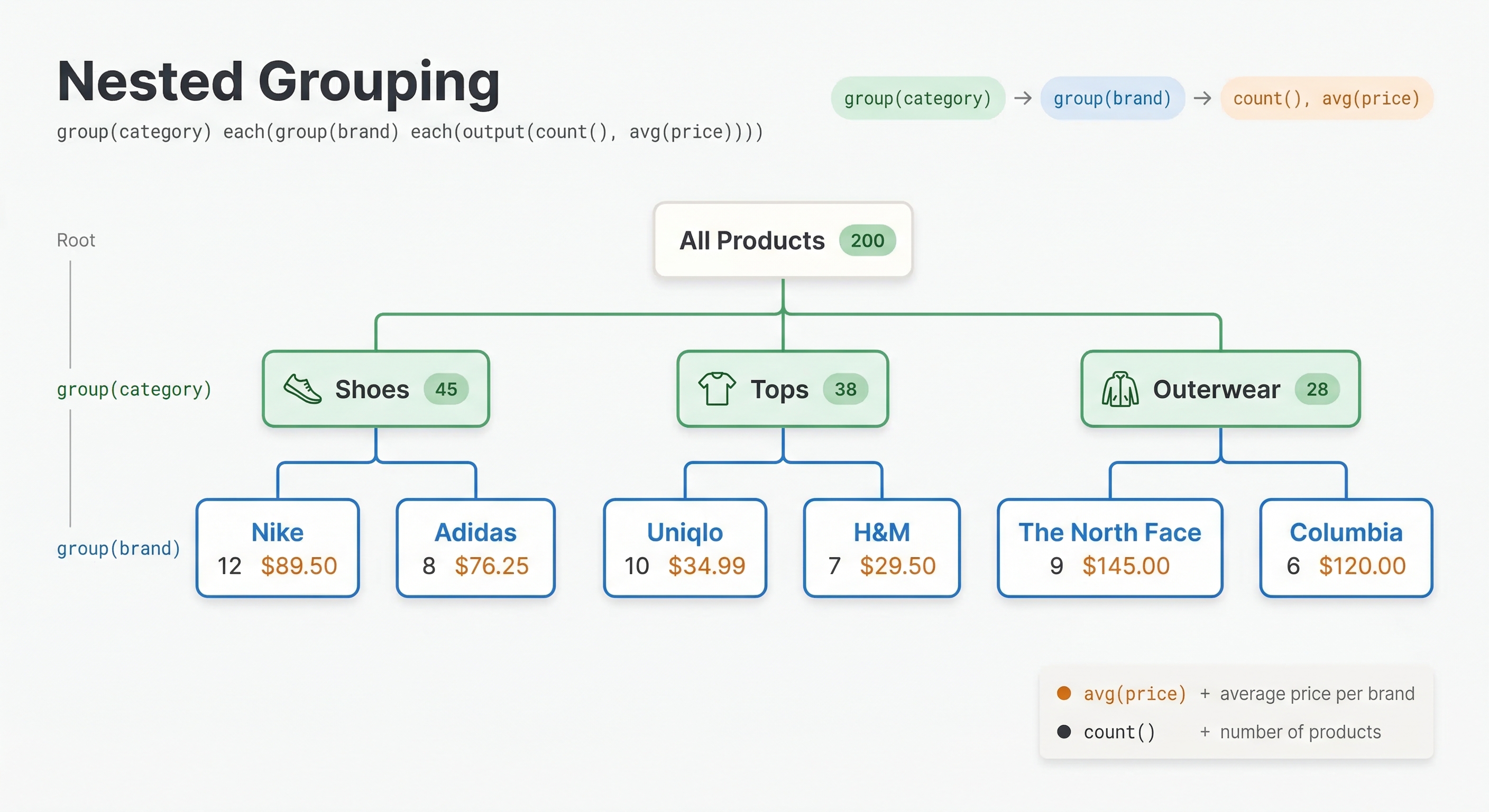
all(group(category) each(group(brand) each(output(count()))))

This first groups by category, then within each category groups by brand, producing a nested structure showing how many documents exist for each category-brand combination.

Ordering Groups

The order() function controls how groups are sorted:

all(group(category) order(-count()) each(output(count())))

The -count() orders by count descending. Use count() without the minus for ascending order. You can order by any aggregation:

all(group(brand) order(-avg(attribute(rating))) each(output(avg(attribute(rating)))))

This orders brands by average rating, showing highest-rated brands first.

Limiting Results

Use max(n) to limit how many groups or documents are returned:

all(group(category) max(20) each(output(count())))

This returns at most 20 categories. Without max(), you might get hundreds of groups, which could be too many for a user interface.

You can limit both groups and documents within groups:

all(group(category) max(10) each(max(5) each(output(summary()))))

This returns 10 categories with 5 documents each.

Labeling Output

You can label grouping results for easier parsing:

all(group(category) each(output(count())) as(category_facets))

The as() function assigns a label. In the JSON response, this grouping appears under the label "category_facets", making it easy to find programmatically.

Continuous Values and Bucketing

For continuous numeric fields, you often want to group into ranges rather than by exact values. Use expressions to create buckets:

all(group(attribute(price) / 100) each(output(count())))

This groups prices into $100 buckets. A product at $245 goes into the bucket 2 (245/100 = 2), effectively the $200-$299 range.

For time-based grouping:

all(group(time.year(attribute(publish_date))) each(output(count())))

This groups by publication year using the time.year() function that extracts the year from a timestamp. Other time functions include time.monthofyear, time.dayofmonth, and time.hourofday for finer granularity.

Combining Grouping with Ranking

Grouping operates on search results after ranking. The ranking function determines which documents match and their order, then grouping organizes those results.

You can use grouping to analyze your ranking:

select * from product where userInput(@query) ranking=my_profile |
all(group(attribute(category)) order(-avg(relevance())) each(output(avg(relevance()))))

The relevance() function accesses each document's rank score. This query shows average relevance scores by category, helping you understand if certain categories systematically rank higher or lower.

Practical Examples

E-commerce facets:

select * from product where userInput(@query) |
all(group(brand) max(20) order(-count()) each(output(count()))) |
all(group(price / 50) max(20) each(output(count()))) |
all(group(rating) each(output(count())))

This provides brand facets, price range facets (in $50 increments), and rating distribution.

News article analytics:

select * from article where publish_date > now() - 86400 |
all(group(time.hourofday(attribute(publish_date))) each(output(count())))

This shows how many articles were published in each hour of the last 24 hours.

Category navigation:

select * from product where category contains "electronics" |
all(group(subcategory) max(20) order(-count()) each(max(3) output(summary())))

This shows subcategories within electronics, with 3 example products per subcategory for browsing.

Performance Considerations

Grouping is computed after retrieval, so it operates on the documents that match your query and pass initial ranking. If your query matches millions of documents, grouping those documents can be expensive.

Use filters to reduce the result set before grouping. Grouping 100,000 documents is manageable. Grouping 10 million can slow queries.

Limit the number of groups with max(). Computing statistics for thousands of unique values takes longer than for dozens.

Choose appropriate rerank counts. If you only need statistics (not documents), you do not need to rank every match. A reasonable first-phase ranking followed by grouping often works well.

Next Steps

You now understand grouping and aggregations for building faceted search and analytics. The next chapter is a hands-on lab where you will add business metrics to ranking and implement grouping queries.

For complete grouping syntax, see the grouping guide and grouping reference.